Warfarin PKPD
Nick Holford, Tomoo Funaki
1 Libraries
The first step is to load the libraries we need - in this case, nlmixr and xpose.nlmixr. (We need RxODE and xpose as well, but those are loaded automatically by nlmixr.)
#Parameters
issim=3 # flag for data source: original data (0, simulated data lag time (1), simulated data transit (2) and (3)
ispds=F # flag to use SAEM (T) or FOCEI (F) for EBEs of PK parameters
isplot=0 # flag to show nlmixr diagnostic and residual plots (1) or not (0)

## Getting started
#Advice from nlmixr installation-notes.rtf (nlmixr_1.1.1-3)
#Make sure there is only one library path
.libPaths()
#> [1] "M:/Apps/R/R-4.0.5/library"
.libPaths(.libPaths()[regexpr("nlmixr",.libPaths())!=-1])
srclib=.libPaths() #srclib="M:\\Apps\\R\\R-4.0.5\\library"

## requires patchwork and xpose.nlmixr packages for markdown.

library(ggplot2,lib=srclib)
library(nlmixr,lib=srclib)
library(RxODE,lib=srclib)
#> RxODE 1.0.8 using 3 threads (see ?getRxThreads)
#>   no cache: create with `rxCreateCache()`
library(xpose,lib=srclib)
#>
#> Attaching package: 'xpose'
#> The following object is masked from 'package:nlmixr':
#>
#>     vpc
#> The following object is masked from 'package:stats':
#>
#>     filter
library(xpose.nlmixr,lib=srclib)
#>
#> Attaching package: 'xpose.nlmixr'
#> The following object is masked from 'package:xpose':
#>
#>     vpc
library(patchwork,lib=srclib)

#Show versions
packageVersion("vpc")
#> [1] '1.2.2'
packageVersion("RxODE")
#> [1] '1.0.8'
nlmixrver=packageVersion("nlmixr")
nlmixrver
#> [1] '2.0.4'
2 Local functions
myvpc=function(nlmixr.fit,ylab) {
   nlmixr::vpc(nlmixr.fit,n=500, show=list(obs_dv=T,sim_median=T,pi=T), bins = bintimes,
       ylab = ylab, xlab = "Time (hours)", stratify="CMT", scales = "free_y")
}

# Goodness of fit plots using xpose
mygof=function(nlmixr.fit) {
   xp.fit <- xpose_data_nlmixr(nlmixr.fit)
   dvpred  <- dv_vs_pred(xp.fit) + labs(title = NULL, subtitle = NULL, caption = NULL)
   dvipred <- dv_vs_ipred(xp.fit) + labs(title = NULL, subtitle = NULL, caption = NULL)
   cwresidv <- res_vs_idv(xp.fit) + labs(title = NULL, subtitle = NULL, caption = NULL)   # default is CWRES
   cwrespred <- res_vs_pred(xp.fit) + labs(title = NULL, subtitle = NULL, caption = NULL) # default is CWRES
   return (dvpred + dvipred + cwresidv + cwrespred + plot_layout(nrow=2) + plot_annotation(title=NULL))
}
3 Data
Original warfarin PKPD data (O’Reilly et al. 1963, 1968) #O’Reilly RA, Aggeler PM, Leong LS. Studies of the coumarin anticoagulant drugs: The pharmacodynamics of warfarin in man. J Clin Invest. 1963;42(10):1542-51. #O’Reilly RA, Aggeler PM. Studies on coumarin anticoagulant drugs. Initiation of warfarin therapy without a loading dose. Circulation. 1968;38:169-77.
PKPD and turnover model for warfarin. (Holford 1986) #Holford NH. Clinical pharmacokinetics and pharmacodynamics of warfarin. Understanding the dose-effect relationship. Clin Pharmacokinet. 1986;11(6):483-504.
NONMEM PKPD model used to simulate data (Funaki et al. 2018) #Funaki T, Holford N, Fujita S. Population PKPD analysis using nlmixr and NONMEM. Population Approach Group Japan2018.
# Read data
datadir="U:\\Research\\Pharmacometrics\\Users\\Tomoo Funaki\\warfarin\\data"
bintimes=c(seq(0,10,1),seq(12,144,12)) # bins for VPC
if (issim==0) {
   datafile="warfarin_dat.csv"
   rdata_ext=""
}
if (issim==1) {
   datafile="ka1_to_emax1_simln_items.csv"
   rdata_ext="_sim"
}
if (issim==2) {
   datafile="ka1_to_emax1_simtr_10.csv"
   rdata_ext="_simtr"
}

if (issim==3) {
   datafile="ka1_to_emax1_simtr2_10.csv"
   rdata_ext="_simtr2"
}

if (ispds) {
   rdata_ext=paste(rdata_ext,"_PDS",sep="")
} else {
   rdata_ext=paste(rdata_ext,"_PDF",sep="")
}

data <- read.csv(file = paste(datadir,datafile,sep="/"))
data$dv <- as.numeric(as.character(data$dv))
names(data) <- toupper(names(data))
data2 <- data
data2$DV <- ifelse(data2$TIME==0 & data2$DVID==1, NA, data2$DV)
3.1 Plot data
Plot the PK and INR data
ggplot(data2, aes(x=TIME, y=DV)) +
  geom_line(aes(group=ID), col="red") +
  scale_x_continuous("Time (h)") +
  scale_y_continuous("Concentration | Effect") +
  facet_wrap(~DVID, scales = "free_y") +
  labs(title="Warfarin single-dose", subtitle="Concentration | Effect vs. time by individual")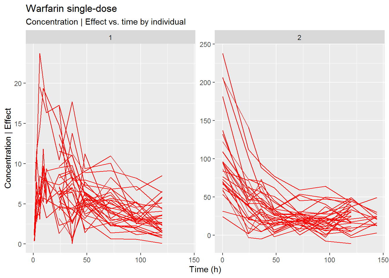
4 PK data
Create PK object from input data
# Selecting only PK data
data.pk <- data[data$DVID==1, ]
data.pk <- data.pk[!is.na(data.pk$DV)|data.pk$AMT!=0, ]
data.pk$CMT <- ifelse(data.pk$AMT!=0, 1, 3)
save(data.pk,file=paste(datadir,"/","datapk",rdata_ext,".RData",sep=""))
#load(paste(datadir,"/",datapk",rdata_ext,".RData",sep=""))
5 PK model
5.1 pk.ka1t PK
Let’s start by fitting the PK model using a 1-compartment model with lag time, first-order absorption and elimination.
pk.ka1t <- function() {
  ini({
    tktr <- log(1)
    tka <- log(1)
    tcl <- log(0.1)
    tv <- log(10)

    eta.ktr ~ 1
    eta.ka ~ 1
    eta.cl ~ 2
    eta.v ~ 1
    eps.pkprop <- 0.1
    eps.pkadd <- 0.1
  })
  model({
    ktr <- exp(tktr + eta.ktr)
    ka <- exp(tka + eta.ka)
    cl <- exp(tcl + eta.cl)
    v <- exp(tv + eta.v)

    d/dt(depot) = -ktr * depot
    d/dt(gut) =  ktr * depot -ka * gut
    d/dt(center) =  ka * gut - cl / v * center

    cp = center / v
    cp ~ prop(eps.pkprop) + add(eps.pkadd)
  })
}
5.1.1 pk.fit.ka1t SAEM
pk.fit.ka1tS <- nlmixr(pk.ka1t, data.pk,  est="saem", control=list(print=0),table=list(cwres=T))
#> [====|====|====|====|====|====|====|====|====|====] 0:00:00
#>
#> [====|====|====|====|====|====|====|====|====|====] 0:00:00
#>
#> [====|====|====|====|====|====|====|====|====|====] 0:00:00
#>
#> [====|====|====|====|====|====|====|====|====|====] 0:00:00
#>
#> [====|====|====|====|====|====|====|====|====|====] 0:00:00
pk.fit.ka1tS
#> -- nlmixr SAEM(ODE); OBJF by FOCEi approximation fit -------------------------------------------------------------------
#>
#>          OBJF      AIC      BIC Log-likelihood Condition Number
#> FOCEi 613.922 1095.229 1130.484      -537.6145         409.7203
#>
#> -- Time (sec pk.fit.ka1tS$time): ---------------------------------------------------------------------------------------
#>
#>          saem  setup table cwres covariance other
#> elapsed 32.57 38.226  0.13 38.42       0.09 7.864
#>
#> -- Population Parameters (pk.fit.ka1tS$parFixed or pk.fit.ka1tS$parFixedDf): -------------------------------------------
#>
#>              Est.     SE      %RSE Back-transformed(95%CI) BSV(CV%) Shrink(SD)%
#> tktr         -0.3   1.14       379    0.741 (0.0798, 6.88)     24.6      78.9%
#> tka        -0.119   1.25 1.05e+003    0.888 (0.0765, 10.3)     31.4      76.9%
#> tcl         -2.24 0.0891      3.97   0.106 (0.0892, 0.126)     41.2      15.2%
#> tv           2.39  0.087      3.64        10.9 (9.2, 12.9)     43.3      12.1%
#> eps.pkprop  0.349                                    0.349
#> eps.pkadd    0.19                                     0.19
#>
#>   Covariance Type (pk.fit.ka1tS$covMethod): linFim
#>   Some strong fixed parameter correlations exist (pk.fit.ka1tS$cor) :
#>     cor:tka,tktr cor:tcl,tktr  cor:tv,tktr  cor:tcl,tka   cor:tv,tka   cor:tv,tcl
#>      -0.982      -0.0714       0.0580       0.0528      -0.0321       -0.103
#>
#>
#>   No correlations in between subject variability (BSV) matrix
#>   Full BSV covariance (pk.fit.ka1tS$omega)
#>     or correlation ( pk.fit.ka1tS $omegaR ; diagonals=SDs)
#>   Distribution stats (mean/skewness/kurtosis/p-value) available in $shrink
#>
#> -- Fit Data (object pk.fit.ka1tS is a modified tibble): ----------------------------------------------------------------
#> # A tibble: 251 x 25
#>   ID     TIME    DV  PRED    RES   WRES IPRED   IRES  IWRES CPRED   CRES  CWRES
#>   <fct> <dbl> <dbl> <dbl>  <dbl>  <dbl> <dbl>  <dbl>  <dbl> <dbl>  <dbl>  <dbl>
#> 1 1       0.5 0.338 0.576 -0.238 -0.575 0.504 -0.165 -0.639 0.572 -0.234 -0.624
#> 2 1       1   0.784 1.78  -0.996 -0.898 1.58  -0.792 -1.36  1.77  -0.985 -0.994
#> 3 1       2   5.09  4.37   0.717  0.283 3.97   1.12   0.803 4.36   0.732  0.316
#> # ... with 248 more rows, and 13 more variables: eta.ktr <dbl>, eta.ka <dbl>,
#> #   eta.cl <dbl>, eta.v <dbl>, depot <dbl>, gut <dbl>, center <dbl>, ktr <dbl>,
#> #   ka <dbl>, cl <dbl>, v <dbl>, tad <dbl>, dosenum <dbl>
if (isplot) plot(pk.fit.ka1tS)
#bootstrapFit(pk.fit.ka1tS, nboot = 100, restart = TRUE) # for illustration but this takes a very long time
5.1.2 pk.fit.ka1t VPC and GOF
The PK VPC using the original data does not describe the peak very well. Hard to see a problem with standard diagnostics.
vpc=myvpc(pk.fit.ka1tS,ylab="PK Concentration (mg/L) saem")
#> [====|====|====|====|====|====|====|====|====|====] 0:00:03

gof=mygof(pk.fit.ka1tS)

vpc/gof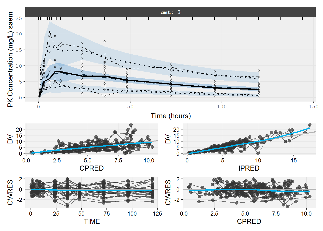
5.1.3 pk.fit.ka1t FOCEI
pk.fit.ka1tF <- nlmixr(pk.ka1t, data.pk,  est="focei", control=list(print=0,outerOpt="bobyqa",table=list(cwres=T)))
#> [====|====|====|====|====|====|====|====|====|====] 0:00:00
#>
#> [====|====|====|====|====|====|====|====|====|====] 0:00:00
#>
#> [====|====|====|====|====|====|====|====|====|====] 0:00:00
#>
#> [====|====|====|====|====|====|====|====|====|====] 0:00:00
#>
#> [====|====|====|====|====|====|====|====|====|====] 0:00:00
#>
#> [====|====|====|====|====|====|====|====|====|====] 0:00:00
#>
#> [====|====|====|====|====|====|====|====|====|====] 0:00:00
#>
#> [====|====|====|====|====|====|====|====|====|====] 0:00:00
#>
#> calculating covariance matrix
#> [====|====|====|====|====|====|====|====|====|====] 0:00:11
#> done
pk.fit.ka1tF
#> -- nlmixr FOCEi (outer: bobyqa) fit ------------------------------------------------------------------------------------
#>
#>           OBJF      AIC      BIC Log-likelihood Condition Number
#> FOCEi 606.1466 1087.454 1122.708      -533.7269         41.21103
#>
#> -- Time (sec pk.fit.ka1tF$time): ---------------------------------------------------------------------------------------
#>
#>          setup optimize covariance table other
#> elapsed 55.284   11.828     11.828  0.08 33.74
#>
#> -- Population Parameters (pk.fit.ka1tF$parFixed or pk.fit.ka1tF$parFixedDf): -------------------------------------------
#>
#>             Est.     SE %RSE Back-transformed(95%CI) BSV(CV%) Shrink(SD)%
#> tktr       0.267  0.128 47.9       1.31 (1.02, 1.68)     10.0      89.6%
#> tka        -0.67  0.089 13.3     0.512 (0.43, 0.609)     10.1      84.4%
#> tcl         -2.2 0.0224 1.02     0.11 (0.106, 0.115)     42.9      13.2%
#> tv          2.39 0.0695  2.9       10.9 (9.54, 12.5)     46.3      8.19%
#> eps.pkprop 0.332                               0.332
#> eps.pkadd  0.144                               0.144
#>
#>   Covariance Type (pk.fit.ka1tF$covMethod): r,s
#>   Fixed parameter correlations in pk.fit.ka1tF$cor
#>   No correlations in between subject variability (BSV) matrix
#>   Full BSV covariance (pk.fit.ka1tF$omega)
#>     or correlation ( pk.fit.ka1tF $omegaR ; diagonals=SDs)
#>   Distribution stats (mean/skewness/kurtosis/p-value) available in $shrink
#>   Minimization message (pk.fit.ka1tF$message):
#>     Normal exit from bobyqa
#>
#> -- Fit Data (object pk.fit.ka1tF is a modified tibble): ----------------------------------------------------------------
#> # A tibble: 251 x 25
#>   ID     TIME    DV  PRED    RES   WRES IPRED   IRES  IWRES CPRED   CRES  CWRES
#>   <fct> <dbl> <dbl> <dbl>  <dbl>  <dbl> <dbl>  <dbl>  <dbl> <dbl>  <dbl>  <dbl>
#> 1 1       0.5 0.338 0.569 -0.230 -0.655 0.535 -0.197 -0.862 0.568 -0.229 -0.686
#> 2 1       1   0.784 1.72  -0.937 -0.961 1.63  -0.843 -1.51  1.72  -0.934 -1.01
#> 3 1       2   5.09  4.14   0.952  0.415 3.95   1.15   0.870 4.13   0.956  0.437
#> # ... with 248 more rows, and 13 more variables: eta.ktr <dbl>, eta.ka <dbl>,
#> #   eta.cl <dbl>, eta.v <dbl>, depot <dbl>, gut <dbl>, center <dbl>, ktr <dbl>,
#> #   ka <dbl>, cl <dbl>, v <dbl>, tad <dbl>, dosenum <dbl>
if (isplot) plot(pk.fit.ka1tF)
5.1.4 pk.fit.ka1t VPC & GOF
The PK VPC using the original data does not describe the peak very well. Hard to see a problem with standard diagnostics.
vpc=myvpc(pk.fit.ka1tF,ylab="PK Concentration (mg/L) focei")
#> [====|====|====|====|====|====|====|====|====|====] 0:00:01

gof=mygof(pk.fit.ka1tF)

vpc/gof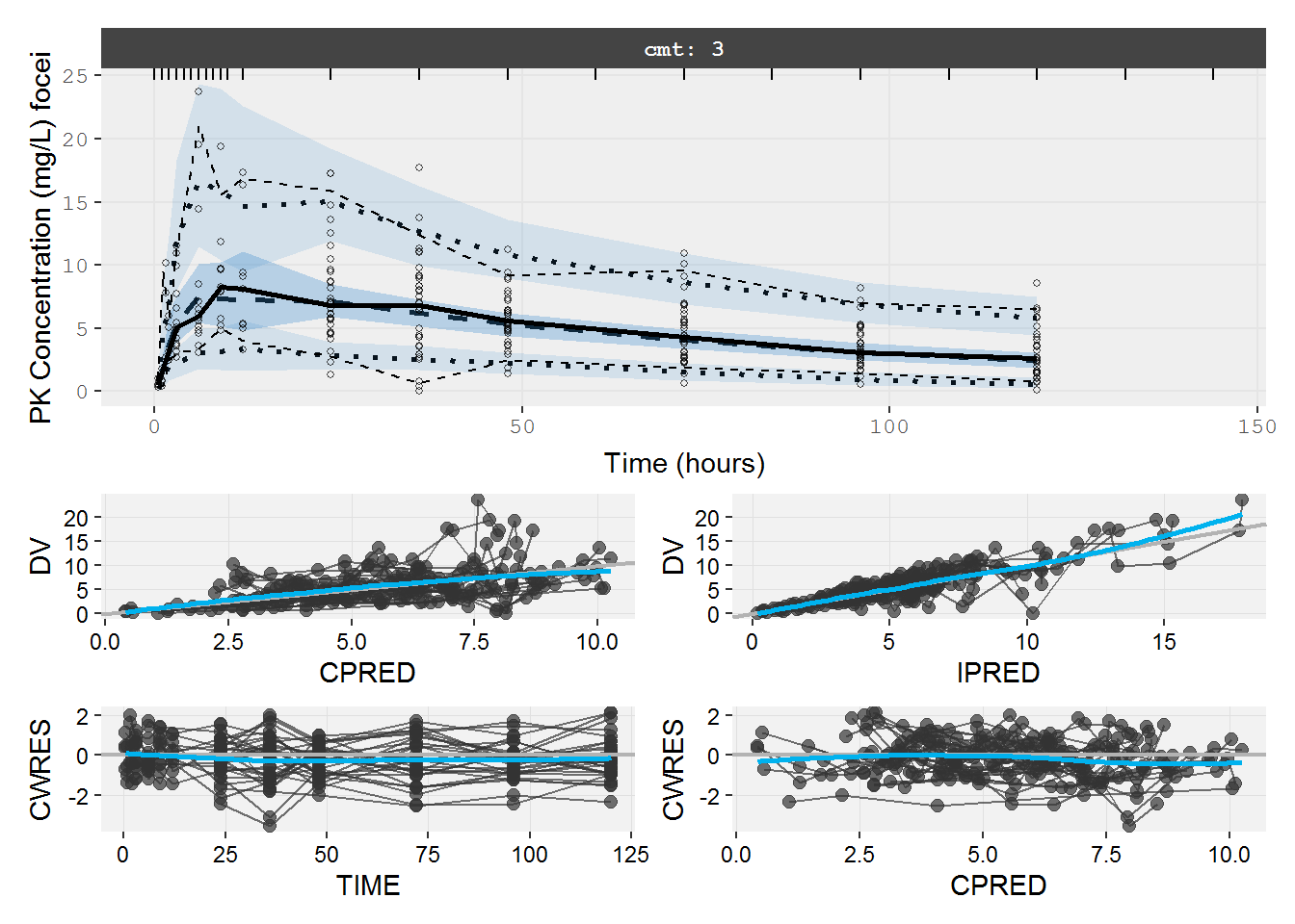
6 PD data
6.1 PD data object with PK EBEs
The PK model empirical Bayes estimates are combined with the effect data to allow a sequential PKPD model.
# Make PD data with SAEM (ispds=1) or FOCEI (ispds=0) EBEs for PK parameters
if (ispds) {
   fit.ipara <- pk.fit.ka1tS[pk.fit.ka1tS$TIME==24,]
} else {
}
#> NULL
   fit.ipara <- pk.fit.ka1tF[pk.fit.ka1tF$TIME==24,]

fit.ipara <- fit.ipara[c("ID", "ktr", "ka", "cl", "v")]
names(fit.ipara) <- c("ID", "IKTR", "IKA", "ICL", "IV")

data.pd <- data
data.pd <- merge(data.pd, fit.ipara, by="ID", all=T)

data.pd$CMT <- ifelse(data.pd$AMT!=0, 1,
                ifelse(data.pd$DVID==2 & data.pd$AMT==0, 4, 3))

#Create MDV=1 for dose record or when DV is recorded as zero
data.pd$MDV <- ifelse(data.pd$AMT>0 | data.pd$DV==0, 1, 0)
#select dosing records and PCA effect records
data.pd <- data.pd[data.pd$AMT!=0 | data.pd$DVID==2, ]

save(data.pd,file=paste(datadir,"/","datapd",rdata_ext,".RData",sep=""))
#load(file=paste(datadir,"/","datapd",rdata_ext,".RData",sep=""))
6.2 PKPD data object
The PKPD data object includes both concentration and effect observations.
data.pkpd <- read.csv(file = paste(datadir,datafile,sep="/"))
names(data.pkpd) = toupper(names(data.pkpd))
data.pkpd$CMT <- data.pkpd$DVID + 2 # DVID 0->2 (center);DVID 2->3 (center); DVID 3->4 (effect)
data.pkpd$CMT[data.pkpd$AMT != 0] <- 1 # CMT 2->1
data.pkpd$EVID[data.pkpd$AMT != 0] <- 101

save(data.pkpd,file=paste(datadir,"/","datapkpd",rdata_ext,".RData",sep=""))
#load(file=paste(datadir,"/","datapkpd",rdata_ext,".RData",sep=""))
7 Sequential PD Models
7.1 pd.cp.logit Immediate PD logit
Sequential immediate effect model - logit for Emax
# define the models
pd.cp.logit <- function() {
  ini({
    poplogit <- 7.5
    tc50 <- log(0.5)
    te0 <- log(100)

    eta.emax ~ .5
    eta.c50  ~ .5
    eta.e0 ~ .5

    eps.pdadd <- 100
  })
  model({
    logit=poplogit+eta.emax
    emax = 1/(1+exp(-logit))
    c50 =  exp(tc50 + eta.c50)
    e0 = exp(te0 + eta.e0)

    # PK parameters from input dataset
    ktr = IKTR
    ka = IKA
    cl = ICL
    v = IV

    cp = center/v

    d/dt(depot) = -ktr * depot
    d/dt(gut) =  ktr * depot -ka * gut
    d/dt(center) =  ka * gut - cl / v * center

    effect=e0*(1-emax*cp/(c50+cp))

    effect ~ add(eps.pdadd)
  })
}
7.1.1 pd.fit.CPS SAEM
#> [====|====|====|====|====|====|====|====|====|====] 0:00:00
#>
#> [====|====|====|====|====|====|====|====|====|====] 0:00:00
#>
#> [====|====|====|====|====|====|====|====|====|====] 0:00:00
#>
#> [====|====|====|====|====|====|====|====|====|====] 0:00:00
#>
#> [====|====|====|====|====|====|====|====|====|====] 0:00:00
#>
#> [1] "IKTR" "IKA"  "ICL"  "IV"
#> -- nlmixr SAEM(ODE); OBJF by FOCEi approximation fit -------------------------------------------------------------------
#>
#>           OBJF      AIC     BIC Log-likelihood Condition Number
#> FOCEi 1689.296 2129.683 2153.81      -1057.842         6.406401
#>
#> -- Time (sec pd.fit.CPS$time): -----------------------------------------------------------------------------------------
#>
#>          saem  setup table cwres covariance other
#> elapsed 40.78 45.655  0.08 45.81       0.06 6.055
#>
#> -- Population Parameters (pd.fit.CPS$parFixed or pd.fit.CPS$parFixedDf): -----------------------------------------------
#>
#>             Est.     SE %RSE Back-transformed(95%CI) BSV(CV% or SD) Shrink(SD)%
#> poplogit     1.4  0.144 10.3        1.4 (1.12, 1.69)          0.485      49.2%
#> tc50      -0.547 0.0574 10.5    0.579 (0.517, 0.648)           20.4      82.1%
#> te0         4.47 0.0816 1.82        87.3 (74.4, 102)           43.3      9.31%
#> eps.pdadd   19.8                                19.8
#>
#>   Covariance Type (pd.fit.CPS$covMethod): linFim
#>   Fixed parameter correlations in pd.fit.CPS$cor
#>   No correlations in between subject variability (BSV) matrix
#>   Full BSV covariance (pd.fit.CPS$omega)
#>     or correlation ( pd.fit.CPS $omegaR ; diagonals=SDs)
#>   Distribution stats (mean/skewness/kurtosis/p-value) available in $shrink
#>
#> -- Fit Data (object pd.fit.CPS is a modified tibble): ------------------------------------------------------------------
#> # A tibble: 232 x 33
#>   ID     TIME    DV  PRED   RES  WRES IPRED  IRES IWRES CPRED  CRES CWRES
#>   <fct> <dbl> <dbl> <dbl> <dbl> <dbl> <dbl> <dbl> <dbl> <dbl> <dbl> <dbl>
#> 1 1        24  73.5  22.5  51.0 2.24   24.4  49.0 2.47   22.4  51.1 2.19
#> 2 1        36  66.0  23.1  42.9 1.87   25.0  41.0 2.07   23.1  42.9 1.84
#> 3 1        48  45.4  23.9  21.5 0.935  25.7  19.7 0.992  23.8  21.6 0.919
#> # ... with 229 more rows, and 21 more variables: eta.emax <dbl>, eta.c50 <dbl>,
#> #   eta.e0 <dbl>, depot <dbl>, gut <dbl>, center <dbl>, logit <dbl>,
#> #   emax <dbl>, c50 <dbl>, e0 <dbl>, ktr <dbl>, ka <dbl>, cl <dbl>, v <dbl>,
#> #   cp <dbl>, tad <dbl>, dosenum <dbl>, IV <dbl>, ICL <dbl>, IKA <dbl>,
#> #   IKTR <dbl>
7.1.2 pd.fit.CPS VPC & GOF
The VPC and GOF plots shows the immediate effect model describes the data poorly.
vpc=myvpc(pd.fit.CPS,ylab="CPS Response (PCA) saem")
#> [====|====|====|====|====|====|====|====|====|====] 0:00:03

gof=mygof(pd.fit.CPS)

vpc/gof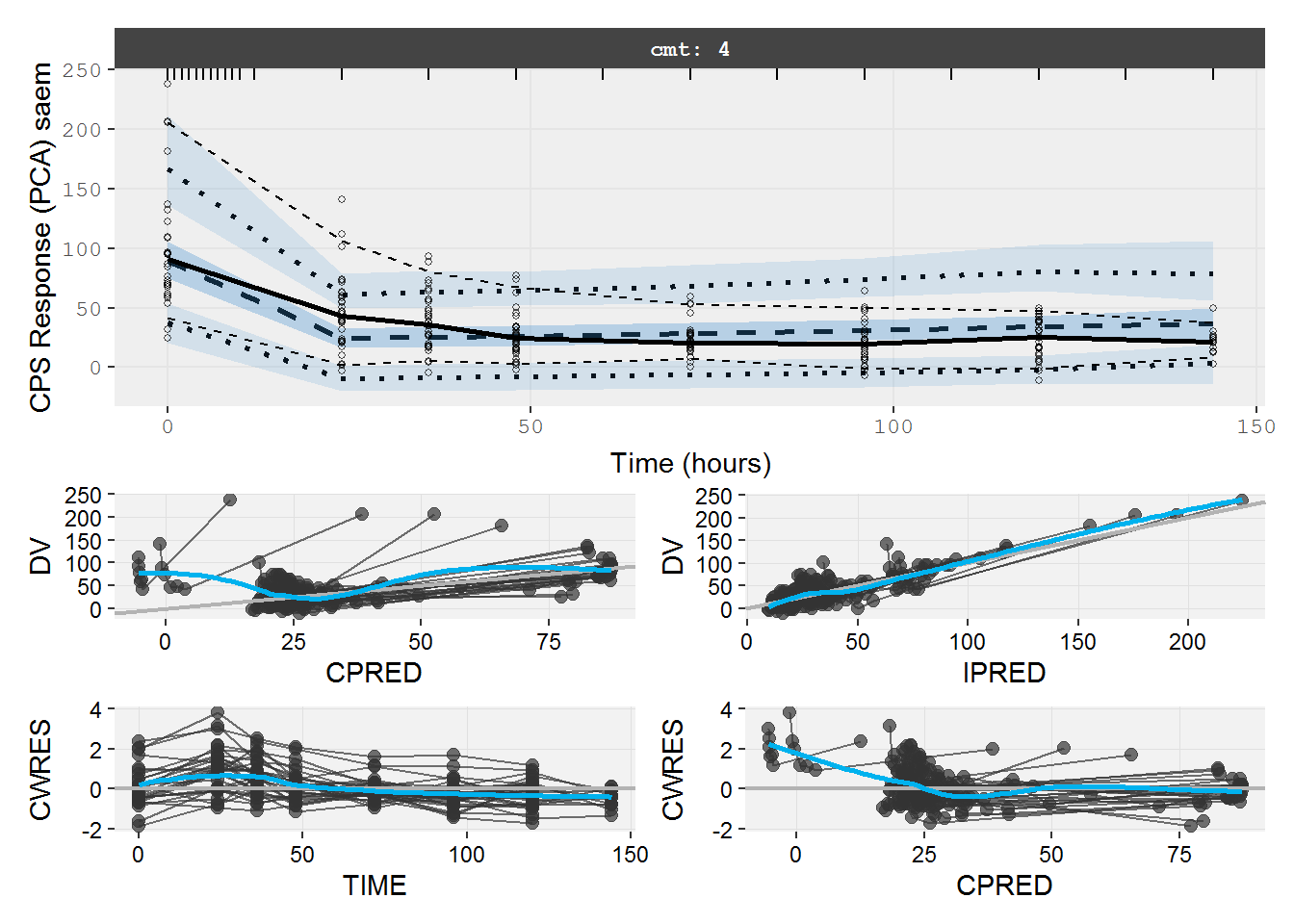
7.2 pd.ce.logit Effect CMT PD logit
Sequential effect compartment model - logit for Emax
pd.ce.logit <- function() {
  ini({
    poplogit <- 7.5
    tc50 <- log(0.5)
    tkout <- log(0.05)
    te0 <- log(100)

    eta.emax ~ .5
    eta.c50  ~ .5
    eta.kout ~ .5
    eta.e0 ~ .5

    eps.pdadd <- 100
  })
  model({
    logit=poplogit+eta.emax
    emax = 1/(1+exp(-logit))
    c50 =  exp(tc50 + eta.c50)
    kout = exp(tkout + eta.kout)
    e0 = exp(te0 + eta.e0)

    # PK parameters from input dataset
    ktr = IKTR
    ka = IKA
    cl = ICL
    v = IV

    cp = center/v

    d/dt(depot) = -ktr * depot
    d/dt(gut) =  ktr * depot -ka * gut
    d/dt(center) =  ka * gut - cl / v * center

    d/dt(ce) = kout*(cp - ce)

    effect=e0*(1-emax*ce/(c50+ce))

    effect ~ add(eps.pdadd)
  })
}
7.2.1 pd.fit.CES SAEM
pd.fit.CES <- nlmixr(pd.ce.logit, data.pd,  est="saem", control=list(print=0),table=list(cwres=T))
#> [====|====|====|====|====|====|====|====|====|====] 0:00:00
#>
#> [====|====|====|====|====|====|====|====|====|====] 0:00:00
#>
#> [====|====|====|====|====|====|====|====|====|====] 0:00:00
#>
#> [====|====|====|====|====|====|====|====|====|====] 0:00:00
#>
#> [====|====|====|====|====|====|====|====|====|====] 0:00:00
#>
#> [1] "IKTR" "IKA"  "ICL"  "IV"
if (isplot) plot(pd.fit.CES)
pd.fit.CES
#> -- nlmixr SAEM(ODE); OBJF by FOCEi approximation fit -------------------------------------------------------------------
#>
#>           OBJF      AIC      BIC Log-likelihood Condition Number
#> FOCEi 1534.141 1978.528 2009.549       -980.264         573.5914
#>
#> -- Time (sec pd.fit.CES$time): -----------------------------------------------------------------------------------------
#>
#>          saem setup table cwres covariance other
#> elapsed 75.11 47.71   0.1  47.9       0.08  5.93
#>
#> -- Population Parameters (pd.fit.CES$parFixed or pd.fit.CES$parFixedDf): -----------------------------------------------
#>
#>             Est.     SE %RSE    Back-transformed(95%CI) BSV(CV% or SD)
#> poplogit    9.85   1.46 14.9          9.85 (6.98, 12.7)           1.63
#> tc50      -0.676 0.0738 10.9        0.508 (0.44, 0.587)           18.3
#> tkout      -5.53  0.146 2.64 0.00397 (0.00298, 0.00528)           51.1
#> te0         4.51 0.0833 1.85           90.9 (77.2, 107)           45.9
#> eps.pdadd   12.7                                   12.7
#>           Shrink(SD)%
#> poplogit       91.8%
#> tc50           67.9%
#> tkout          29.6%
#> te0            4.07%
#> eps.pdadd
#>
#>   Covariance Type (pd.fit.CES$covMethod): linFim
#>   Fixed parameter correlations in pd.fit.CES$cor
#>   No correlations in between subject variability (BSV) matrix
#>   Full BSV covariance (pd.fit.CES$omega)
#>     or correlation ( pd.fit.CES $omegaR ; diagonals=SDs)
#>   Distribution stats (mean/skewness/kurtosis/p-value) available in $shrink
#>
#> -- Fit Data (object pd.fit.CES is a modified tibble): ------------------------------------------------------------------
#> # A tibble: 232 x 36
#>   ID     TIME    DV  PRED   RES  WRES IPRED  IRES IWRES CPRED  CRES CWRES
#>   <fct> <dbl> <dbl> <dbl> <dbl> <dbl> <dbl> <dbl> <dbl> <dbl> <dbl> <dbl>
#> 1 1        24  73.5  40.2  33.3 1.37   54.9 18.6  1.46   37.8  35.7 1.16
#> 2 1        36  66.0  32.3  33.7 1.57   44.3 21.7  1.70   30.3  35.7 1.33
#> 3 1        48  45.4  27.8  17.6 0.887  38.2  7.14 0.561  26.1  19.3 0.792
#> # ... with 229 more rows, and 24 more variables: eta.emax <dbl>, eta.c50 <dbl>,
#> #   eta.kout <dbl>, eta.e0 <dbl>, depot <dbl>, gut <dbl>, center <dbl>,
#> #   ce <dbl>, logit <dbl>, emax <dbl>, c50 <dbl>, kout <dbl>, e0 <dbl>,
#> #   ktr <dbl>, ka <dbl>, cl <dbl>, v <dbl>, cp <dbl>, tad <dbl>, dosenum <dbl>,
#> #   IV <dbl>, ICL <dbl>, IKA <dbl>, IKTR <dbl>
7.2.2 pd.fit.CES VPC & GOF
The VPC and GOF show the effect compartment model does not describe the data well.
vpc=myvpc(pd.fit.CES,ylab="CES Response (PCA) saem")
#> [====|====|====|====|====|====|====|====|====|====] 0:00:02

gof=mygof(pd.fit.CES)

vpc/gof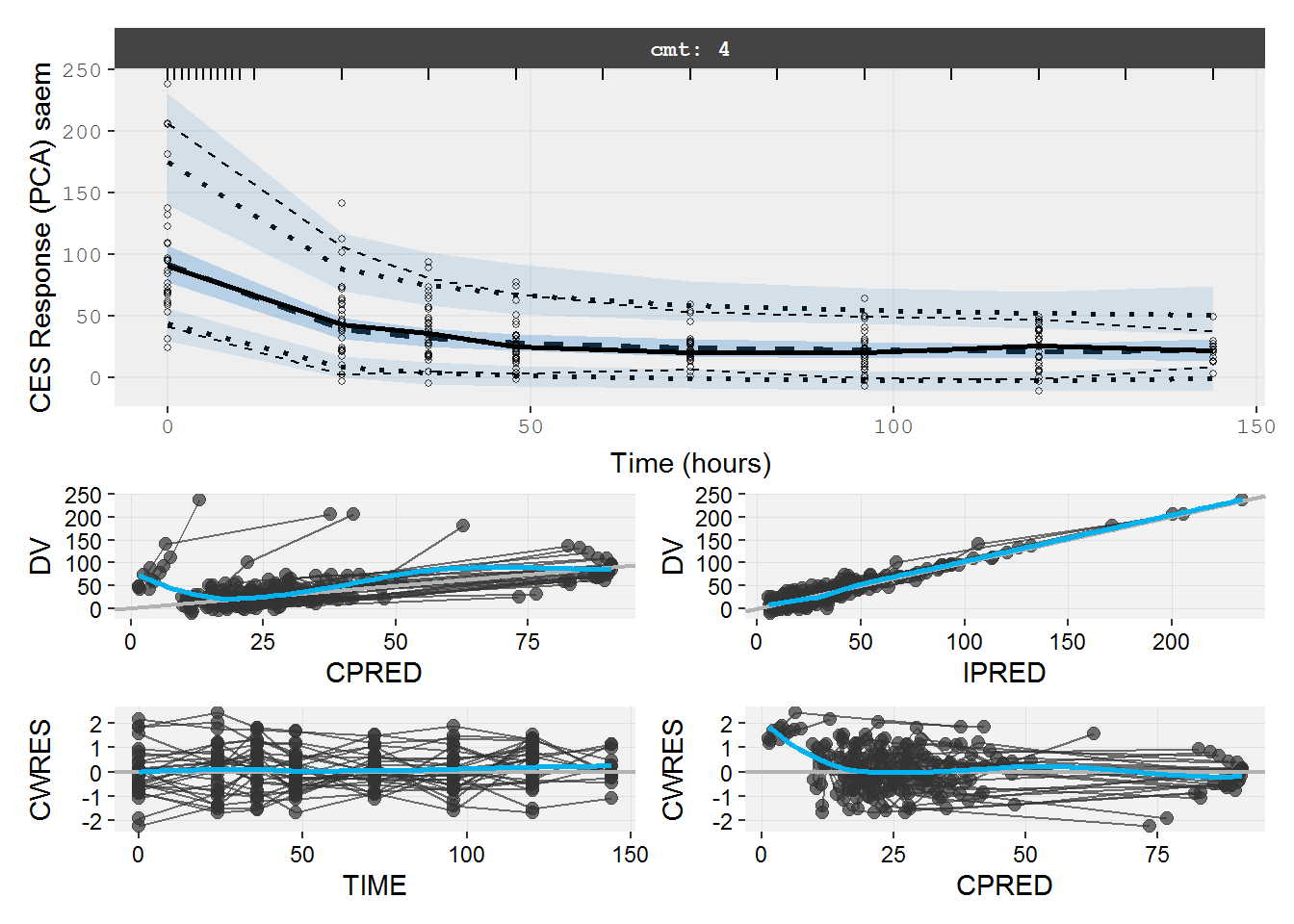
7.3 pd.turnover.logit Turnover PD logit
Sequential turnover model - logit for Emax
pd.turnover.logit <- function() { # The logit transformation is used to constrain Emax in SAEM
  ini({
    poplogit <- 7.5
    tc50 <- log(0.5)
    tkout <- log(0.05)
    te0 <- log(100)

    eta.emax ~ .5
    eta.c50  ~ .5
    eta.kout ~ .5
    eta.e0 ~ .5

    eps.pdadd <- 100
  })
  model({
    logit=poplogit+eta.emax
    emax = 1/(1+exp(-logit))
    c50 =  exp(tc50 + eta.c50)
    kout = exp(tkout + eta.kout)
    e0 = exp(te0 + eta.e0)

    # PK parameters from input dataset
    ktr = IKTR
    ka = IKA
    cl = ICL
    v = IV

    cp = center/v

    PD=1-emax*cp/(c50+cp)

    effect(0) = e0
    kin = e0*kout

    d/dt(depot) = -ktr * depot
    d/dt(gut) =  ktr * depot -ka * gut
    d/dt(center) =  ka * gut - cl / v * center

    d/dt(effect) = kin*PD -kout*effect

    effect ~ add(eps.pdadd)
  })
}
7.3.1 pd.fit.TOS SAEM
Sequential turnover model logit
################ Run nlmixr with PD and PKPD models ###########################
pd.fit.TOS <- nlmixr(pd.turnover.logit, data.pd,  est="saem", control=list(print=0),table=list(cwres=T))
#> [====|====|====|====|====|====|====|====|====|====] 0:00:00
#>
#> [====|====|====|====|====|====|====|====|====|====] 0:00:00
#>
#> [====|====|====|====|====|====|====|====|====|====] 0:00:00
#>
#> [====|====|====|====|====|====|====|====|====|====] 0:00:00
#>
#> [====|====|====|====|====|====|====|====|====|====] 0:00:00
#>
#> [1] "IKTR" "IKA"  "ICL"  "IV"
if (isplot) plot(pd.fit.TOS)
pd.fit.TOS
#> -- nlmixr SAEM(ODE); OBJF by FOCEi approximation fit -------------------------------------------------------------------
#>
#>           OBJF      AIC     BIC Log-likelihood Condition Number
#> FOCEi 1507.262 1951.649 1982.67      -966.8246         48.28872
#>
#> -- Time (sec pd.fit.TOS$time): -----------------------------------------------------------------------------------------
#>
#>          saem  setup table cwres covariance other
#> elapsed 62.79 47.356  0.13 47.65       0.06 6.564
#>
#> -- Population Parameters (pd.fit.TOS$parFixed or pd.fit.TOS$parFixedDf): -----------------------------------------------
#>
#>             Est.     SE %RSE Back-transformed(95%CI) BSV(CV% or SD) Shrink(SD)%
#> poplogit    7.53  0.581 7.72       7.53 (6.39, 8.67)           1.55      90.6%
#> tc50      -0.302  0.112   37     0.74 (0.594, 0.921)           48.0      36.2%
#> tkout      -3.31  0.109  3.3 0.0365 (0.0295, 0.0452)           53.0      18.1%
#> te0          4.5 0.0839 1.86        90.4 (76.7, 106)           48.0      3.14%
#> eps.pdadd   10.9                                10.9
#>
#>   Covariance Type (pd.fit.TOS$covMethod): linFim
#>   Fixed parameter correlations in pd.fit.TOS$cor
#>   No correlations in between subject variability (BSV) matrix
#>   Full BSV covariance (pd.fit.TOS$omega)
#>     or correlation ( pd.fit.TOS $omegaR ; diagonals=SDs)
#>   Distribution stats (mean/skewness/kurtosis/p-value) available in $shrink
#>
#> -- Fit Data (object pd.fit.TOS is a modified tibble): ------------------------------------------------------------------
#> # A tibble: 232 x 38
#>   ID     TIME    DV  PRED   RES  WRES IPRED  IRES IWRES CPRED  CRES CWRES
#>   <fct> <dbl> <dbl> <dbl> <dbl> <dbl> <dbl> <dbl> <dbl> <dbl> <dbl> <dbl>
#> 1 1        24  73.5  43.3  30.2  1.11  70.0  3.51 0.322  37.0  36.5 0.938
#> 2 1        36  66.0  31.2  34.8  1.51  53.1 12.9  1.19   24.7  41.3 1.21
#> 3 1        48  45.4  23.7  21.6  1.09  41.0  4.35 0.399  17.4  28.0 0.934
#> # ... with 229 more rows, and 26 more variables: eta.emax <dbl>, eta.c50 <dbl>,
#> #   eta.kout <dbl>, eta.e0 <dbl>, depot <dbl>, gut <dbl>, center <dbl>,
#> #   effect <dbl>, logit <dbl>, emax <dbl>, c50 <dbl>, kout <dbl>, e0 <dbl>,
#> #   ktr <dbl>, ka <dbl>, cl <dbl>, v <dbl>, cp <dbl>, PD <dbl>, kin <dbl>,
#> #   tad <dbl>, dosenum <dbl>, IV <dbl>, ICL <dbl>, IKA <dbl>, IKTR <dbl>
7.3.2 pd.fit.TOS VPC & GOF
The VPC and GOF show the turnover model describes the PD data well.
vpc=myvpc(pd.fit.TOS,ylab="pd TOS Response (PCA) saem")
#> [====|====|====|====|====|====|====|====|====|====] 0:00:03

gof=mygof(pd.fit.TOS)

vpc/gof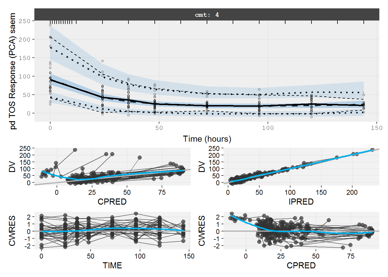
7.4 pd.cp.emax Immediate PD Emax
Sequential immediate effect model Emax<1
pd.cp.emax <- function() {
  ini({
    popemax <- c(0,0.9,0.999)
    tc50 <- log(0.5)
    te0 <- log(100)

    eta.emax ~ .5
    eta.c50  ~ .5
    eta.e0 ~ .5

    eps.pdadd <- 100
  })
  model({
    poplogit = log(popemax/(1-popemax))
    logit=poplogit+eta.emax
    emax = 1/(1+exp(-logit))
    c50 =  exp(tc50 + eta.c50)
    e0 = exp(te0 + eta.e0)

    # PK parameters from input dataset
    ktr = IKTR
    ka = IKA
    cl = ICL
    v = IV

    cp = center/v

    d/dt(depot) = -ktr * depot
    d/dt(gut) =  ktr * depot -ka * gut
    d/dt(center) =  ka * gut - cl / v * center

    effect=e0*(1-emax*cp/(c50+cp))

    effect ~ add(eps.pdadd)
  })
}
7.4.1 pd.fit.CPF FOCEI
#> [====|====|====|====|====|====|====|====|====|====] 0:00:00
#>
#> [====|====|====|====|====|====|====|====|====|====] 0:00:00
#>
#> [====|====|====|====|====|====|====|====|====|====] 0:00:00
#>
#> [====|====|====|====|====|====|====|====|====|====] 0:00:00
#>
#> [====|====|====|====|====|====|====|====|====|====] 0:00:00
#>
#> [====|====|====|====|====|====|====|====|====|====] 0:00:00
#>
#> [====|====|====|====|====|====|====|====|====|====] 0:00:00
#>
#> [====|====|====|====|====|====|====|====|====|====] 0:00:00
#>
#> [1] "IKTR" "IKA"  "ICL"  "IV"
#> calculating covariance matrix
#> [====|====|====|====|====|====|====|====|====|====] 0:00:05
#> done
#> -- nlmixr FOCEi (outer: bobyqa) fit ------------------------------------------------------------------------------------
#>
#>           OBJF      AIC      BIC Log-likelihood Condition Number
#> FOCEi 1646.729 2087.117 2111.244      -1036.558            48709
#>
#> -- Time (sec pd.fit.CPF$time): -----------------------------------------------------------------------------------------
#>
#>          setup optimize covariance table  other
#> elapsed 42.788    5.337      5.337  0.11 58.588
#>
#> -- Population Parameters (pd.fit.CPF$parFixed or pd.fit.CPF$parFixedDf): -----------------------------------------------
#>
#>            Est.     SE %RSE  Back-transformed(95%CI) BSV(CV%) Shrink(SD)%
#> popemax   0.707 0.0308 4.36     0.707 (0.646, 0.767)
#> tc50      -6.43   6.62  103 0.00162 (3.79e-009, 693)     320.      99.2%
#> te0        4.53  0.116 2.56         92.4 (73.6, 116)     43.2      9.26%
#> eps.pdadd  17.5                                 17.5
#>
#> -- BSV Covariance (pd.fit.CPF$omega): ----------------------------------------------------------------------------------
#>           eta.emax  eta.c50    eta.e0
#> eta.emax 0.1362351 0.000000 0.0000000
#> eta.c50  0.0000000 2.422088 0.0000000
#> eta.e0   0.0000000 0.000000 0.1710548
#>
#>   Not all variables are mu-referenced.
#>   Can also see BSV Correlation (pd.fit.CPF$omegaR; diagonals=SDs)
#>   Covariance Type (pd.fit.CPF$covMethod): r
#>   Fixed parameter correlations in pd.fit.CPF$cor
#>   Distribution stats (mean/skewness/kurtosis/p-value) available in $shrink
#>   Minimization message (pd.fit.CPF$message):
#>     Normal exit from bobyqa
#>
#> -- Fit Data (object pd.fit.CPF is a modified tibble): ------------------------------------------------------------------
#> # A tibble: 232 x 34
#>   ID     TIME    DV  PRED   RES  WRES IPRED  IRES IWRES CPRED  CRES CWRES
#>   <fct> <dbl> <dbl> <dbl> <dbl> <dbl> <dbl> <dbl> <dbl> <dbl> <dbl> <dbl>
#> 1 1        24  73.5  27.1  46.4 2.11   32.7  40.8 2.33   26.6  46.9 1.99
#> 2 1        36  66.0  27.1  38.9 1.77   32.7  33.3 1.91   26.6  39.4 1.67
#> 3 1        48  45.4  27.1  18.2 0.832  32.7  12.7 0.725  26.6  18.8 0.794
#> # ... with 229 more rows, and 22 more variables: eta.emax <dbl>, eta.c50 <dbl>,
#> #   eta.e0 <dbl>, depot <dbl>, gut <dbl>, center <dbl>, poplogit <dbl>,
#> #   logit <dbl>, emax <dbl>, c50 <dbl>, e0 <dbl>, ktr <dbl>, ka <dbl>,
#> #   cl <dbl>, v <dbl>, cp <dbl>, tad <dbl>, dosenum <dbl>, IV <dbl>, ICL <dbl>,
#> #   IKA <dbl>, IKTR <dbl>
7.4.2 pd.fit.CPF VPC & GOF
The VPC and GOF shows the immediate effect model does not describe the PD data well.
vpc=myvpc(pd.fit.CPF,ylab="pd CPF Response (PCA) focei")
#> [====|====|====|====|====|====|====|====|====|====] 0:00:02

gof=mygof(pd.fit.CPF)

vpc/gof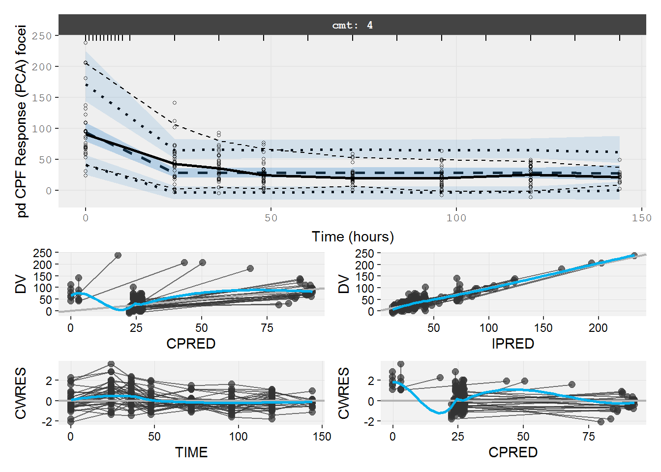
7.5 pd.ce.emax effect CMT Emax
Sequential effect compartment model Emax<1
pd.ce.emax <- function() { #clearer emax parameter constraint method which works with FOCEI
  ini({
    popemax <- c(0,0.9,0.999)
    tc50 <- log(0.5)
    tkout <- log(0.05)
    te0 <- log(100)

    eta.emax ~ .5
    eta.c50  ~ .5
    eta.kout ~ .5
    eta.e0 ~ .5

    eps.pdadd <- 100
  })
  model({
    poplogit = log(popemax/(1-popemax))
    logit=poplogit+eta.emax
    emax = 1/(1+exp(-logit))
    c50 =  exp(tc50 + eta.c50)
    kout = exp(tkout + eta.kout)
    e0 = exp(te0 + eta.e0)

    # PK parameters from input dataset
    ktr = IKTR
    ka = IKA
    cl = ICL
    v = IV

    cp = center/v

    d/dt(depot) = -ktr * depot
    d/dt(gut) =  ktr * depot -ka * gut
    d/dt(center) =  ka * gut - cl / v * center

    d/dt(ce) = kout*(cp - ce)

    effect=e0*(1-emax*ce/(c50+ce))

    effect ~ add(eps.pdadd)
  })
}
7.5.1 pd.fit.CEF FOCEI
################ Effect compartment PD model FOCEI ###########
#   pd.fit.CEF <- nlmixr(pd.ce.emax, data.pd,  est="focei", control=foceiControl(print=100000)) # Default opt method fails
pd.fit.CEF <- nlmixr(pd.ce.emax, data.pd,  est="focei", control=list(print=0,outerOpt="bobyqa",table=list(cwres=T)))
#> [====|====|====|====|====|====|====|====|====|====] 0:00:00
#>
#> [====|====|====|====|====|====|====|====|====|====] 0:00:00
#>
#> [====|====|====|====|====|====|====|====|====|====] 0:00:00
#>
#> [====|====|====|====|====|====|====|====|====|====] 0:00:00
#>
#> [====|====|====|====|====|====|====|====|====|====] 0:00:00
#>
#> [====|====|====|====|====|====|====|====|====|====] 0:00:00
#>
#> [====|====|====|====|====|====|====|====|====|====] 0:00:00
#>
#> [====|====|====|====|====|====|====|====|====|====] 0:00:00
#>
#> [1] "IKTR" "IKA"  "ICL"  "IV"
#> unhandled error message: EE:lsoda -- at t = 8.30738e-009 and step size _C(h) = 3.16901e-014, the
#>  corrector convergence failed repeatedly or
#>  with fabs(_C(h)) = hmin
#>  @(lsoda.c:887)
#> calculating covariance matrix
#> [====|====|====|====|====|====|====|====|===
S matrix calculation failed; Switch to R-matrix covariance.
#> =|====] 0:00:08
#> done
if (isplot) plot(pd.fit.CEF)
pd.fit.CEF
#> -- nlmixr FOCEi (outer: bobyqa) fit ------------------------------------------------------------------------------------
#>
#>         OBJF    AIC    BIC Log-likelihood
#> FOCEi 5e+100 5e+100 5e+100      -2.5e+100
#>
#> -- Time (sec pd.fit.CEF$time): -----------------------------------------------------------------------------------------
#>
#>          setup optimize covariance table  other
#> elapsed 46.547    8.448      8.448  0.15 12.657
#>
#> -- Population Parameters (pd.fit.CEF$parFixed or pd.fit.CEF$parFixedDf): -----------------------------------------------
#>
#>             Est. Back-transformed BSV(CV%) Shrink(SD)%
#> popemax    0.836            0.836
#> tc50      -0.702            0.496     76.4      72.2%
#> tkout         -3           0.0496     79.7     -534.%
#> te0          4.5             89.7     43.3      16.1%
#> eps.pdadd     22               22
#>
#> -- BSV Covariance (pd.fit.CEF$omega): ----------------------------------------------------------------------------------
#>           eta.emax   eta.c50  eta.kout    eta.e0
#> eta.emax 0.3979735 0.0000000 0.0000000 0.0000000
#> eta.c50  0.0000000 0.4600564 0.0000000 0.0000000
#> eta.kout 0.0000000 0.0000000 0.4922557 0.0000000
#> eta.e0   0.0000000 0.0000000 0.0000000 0.1718628
#>
#>   Not all variables are mu-referenced.
#>   Can also see BSV Correlation (pd.fit.CEF$omegaR; diagonals=SDs)
#>   Covariance Type (pd.fit.CEF$covMethod): failed
#>   Distribution stats (mean/skewness/kurtosis/p-value) available in $shrink
#>   Minimization message (pd.fit.CEF$message):
#>     Normal exit from bobyqa
#>
#> -- Fit Data (object pd.fit.CEF is a modified tibble): ------------------------------------------------------------------
#> # A tibble: 232 x 37
#>   ID     TIME    DV  PRED   RES  WRES IPRED  IRES IWRES CPRED  CRES CWRES
#>   <fct> <dbl> <dbl> <dbl> <dbl> <dbl> <dbl> <dbl> <dbl> <dbl> <dbl> <dbl>
#> 1 1        24  73.5  21.4  52.1 2.07   21.4  52.1  2.37  21.4  52.1 2.07
#> 2 1        36  66.0  20.6  45.4 1.81   20.6  45.4  2.06  20.6  45.4 1.81
#> 3 1        48  45.4  20.6  24.8 0.992  20.6  24.8  1.12  20.6  24.8 0.992
#> # ... with 229 more rows, and 25 more variables: eta.emax <dbl>, eta.c50 <dbl>,
#> #   eta.kout <dbl>, eta.e0 <dbl>, depot <dbl>, gut <dbl>, center <dbl>,
#> #   ce <dbl>, poplogit <dbl>, logit <dbl>, emax <dbl>, c50 <dbl>, kout <dbl>,
#> #   e0 <dbl>, ktr <dbl>, ka <dbl>, cl <dbl>, v <dbl>, cp <dbl>, tad <dbl>,
#> #   dosenum <dbl>, IV <dbl>, ICL <dbl>, IKA <dbl>, IKTR <dbl>
7.5.2 pd.fit.CEF VPC & GOF
vpc=myvpc(pd.fit.CEF,ylab="pd CEF Response (PCA) focei")
#> [====|====|====|====|====|====|====|====|====|====] 0:00:00
#>
#> [====|====|====|====|====|====|====|====|====|====] 0:00:00
#>
#> [====|====|====|====|====|====|====|====|====|====] 0:00:01
#>
#> [====|====|====|====|====|====|====|====|====|====] 0:00:00
#>
#> [====|====|====|====|====|====|====|====|====|====] 0:00:00
#>
#> [====|====|====|====|====|====|====|====|====|====] 0:00:00
#>
#> [====|====|====|====|====|====|====|====|====|====] 0:00:00
#>
#> [====|====|====|====|====|====|====|====|====|====] 0:00:00
#>
#> [1] "IKTR" "IKA"  "ICL"  "IV"
#> calculating covariance matrix
#> [====|====|====|====|====|====|====|====|====|====] 0:00:01
#> [====|====|====|====|====|====|====|====|====|====

gof=mygof(pd.fit.CEF)

vpc/gof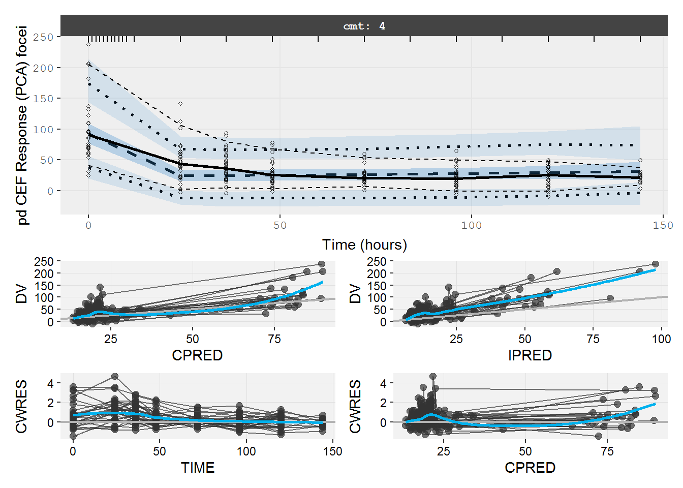
7.6 pd.turnover.emax Turnover PD Emax
Sequential turnover model Emax<1
pd.turnover.emax <- function() {
  ini({
    popemax <- c(0,0.9,0.999)
    tc50 <- log(0.5)
    tkout <- log(0.05)
    te0 <- log(100)

    eta.emax ~ .5
    eta.c50  ~ .5
    eta.kout ~ .5
    eta.e0 ~ .5

    eps.pdadd <- 100
  })
  model({
    poplogit = log(popemax/(1-popemax))
    logit=poplogit+eta.emax
    emax = 1/(1+exp(-logit))
    c50 =  exp(tc50 + eta.c50)
    kout = exp(tkout + eta.kout)
    e0 = exp(te0 + eta.e0)

    # PK parameters from input dataset
    ktr = IKTR
    ka = IKA
    cl = ICL
    v = IV

    cp = center/v

    PD=1-emax*cp/(c50+cp)

    effect(0) = e0
    kin = e0*kout

    d/dt(depot) = -ktr * depot
    d/dt(gut) =  ktr * depot -ka * gut
    d/dt(center) =  ka * gut - cl / v * center

    d/dt(effect) = kin*PD -kout*effect

    effect ~ add(eps.pdadd)
  })
}
7.6.1 pd.fit.TOF FOCEI
################ Turnover (true) PD model FOCEI ###########
pd.fit.TOF <- nlmixr(pd.turnover.emax, data.pd,  est="focei", control=list(print=0,outerOpt="bobyqa",table=list(cwres=T)))
#> [====|====|====|====|====|====|====|====|====|====] 0:00:00
#>
#> [====|====|====|====|====|====|====|====|====|====] 0:00:01
#>
#> [====|====|====|====|====|====|====|====|====|====] 0:00:00
#>
#> [====|====|====|====|====|====|====|====|====|====] 0:00:00
#>
#> [====|====|====|====|====|====|====|====|====|====] 0:00:00
#>
#> [====|====|====|====|====|====|====|====|====|====] 0:00:00
#>
#> [====|====|====|====|====|====|====|====|====|====] 0:00:00
#>
#> [====|====|====|====|====|====|====|====|====|====] 0:00:00
#>
#> [1] "IKTR" "IKA"  "ICL"  "IV"
#> calculating covariance matrix
#> [====|====|====|====|====|====|====|====|====|====] 0:00:27
#> done
if (isplot) plot(pd.fit.TOF)
pd.fit.TOF
#> -- nlmixr FOCEi (outer: bobyqa) fit ------------------------------------------------------------------------------------
#>
#>           OBJF      AIC      BIC Log-likelihood Condition Number
#> FOCEi 1507.147 1951.534 1982.555      -966.7672         296.9303
#>
#> -- Time (sec pd.fit.TOF$time): -----------------------------------------------------------------------------------------
#>
#>          setup optimize covariance table  other
#> elapsed 55.823   27.571     27.571  0.16 74.245
#>
#> -- Population Parameters (pd.fit.TOF$parFixed or pd.fit.TOF$parFixedDf): -----------------------------------------------
#>
#>             Est.     SE %RSE Back-transformed(95%CI) BSV(CV%) Shrink(SD)%
#> popemax    0.925 0.0208 2.25    0.925 (0.884, 0.965)
#> tc50      -0.773  0.234 30.3     0.462 (0.292, 0.73)     46.1      52.2%
#> tkout      -3.21  0.105 3.28 0.0404 (0.0329, 0.0497)     58.2      23.0%
#> te0         4.51 0.0737 1.64        90.5 (78.3, 105)     49.0      7.50%
#> eps.pdadd   10.8                                10.8
#>
#> -- BSV Covariance (pd.fit.TOF$omega): ----------------------------------------------------------------------------------
#>           eta.emax   eta.c50  eta.kout    eta.e0
#> eta.emax 0.5424419 0.0000000 0.0000000 0.0000000
#> eta.c50  0.0000000 0.1927781 0.0000000 0.0000000
#> eta.kout 0.0000000 0.0000000 0.2913137 0.0000000
#> eta.e0   0.0000000 0.0000000 0.0000000 0.2151494
#>
#>   Not all variables are mu-referenced.
#>   Can also see BSV Correlation (pd.fit.TOF$omegaR; diagonals=SDs)
#>   Covariance Type (pd.fit.TOF$covMethod): r,s
#>   Fixed parameter correlations in pd.fit.TOF$cor
#>   Distribution stats (mean/skewness/kurtosis/p-value) available in $shrink
#>   Minimization message (pd.fit.TOF$message):
#>     Normal exit from bobyqa
#>
#> -- Fit Data (object pd.fit.TOF is a modified tibble): ------------------------------------------------------------------
#> # A tibble: 232 x 39
#>   ID     TIME    DV  PRED   RES  WRES IPRED  IRES IWRES CPRED  CRES CWRES
#>   <fct> <dbl> <dbl> <dbl> <dbl> <dbl> <dbl> <dbl> <dbl> <dbl> <dbl> <dbl>
#> 1 1        24  73.5  42.3  31.2  1.13  70.7  2.78 0.256  34.8  38.7 0.950
#> 2 1        36  66.0  30.7  35.3  1.51  53.7 12.4  1.14   23.2  42.9 1.20
#> 3 1        48  45.4  23.9  21.5  1.08  41.7  3.67 0.338  16.6  28.8 0.919
#> # ... with 229 more rows, and 27 more variables: eta.emax <dbl>, eta.c50 <dbl>,
#> #   eta.kout <dbl>, eta.e0 <dbl>, depot <dbl>, gut <dbl>, center <dbl>,
#> #   effect <dbl>, poplogit <dbl>, logit <dbl>, emax <dbl>, c50 <dbl>,
#> #   kout <dbl>, e0 <dbl>, ktr <dbl>, ka <dbl>, cl <dbl>, v <dbl>, cp <dbl>,
#> #   PD <dbl>, kin <dbl>, tad <dbl>, dosenum <dbl>, IV <dbl>, ICL <dbl>,
#> #   IKA <dbl>, IKTR <dbl>
7.6.2 pd.fit.TOF VPC & GOF
Quitting from lines 704-711 (warf_simtr_PKPD_vpc_ui_saem_foce_B-18-v3_PDF.Rmd) Error in foceiFit.data.frame0(data = .dat, inits = .inits, PKpars = .uif$theta.pars, : Could not fit data. Calls:
#vpc=myvpc(pd.fit.TOF,ylab="pd TOF Response (PCA) focei")

#gof=mygof(pd.fit.TOF)

#vpc/gof
8 Joint PKPD models
We can jointly fit the PK and PD data with a single model.
8.1 pkpd.cp.logit Imm PKPD logit
Joint turnover model Emax<1
pkpd.cp.logit <- function() {
  ini({
    tktr <- log(1)
    tka <- log(1)
    tcl <- log(0.1)
    tv <- log(10)

    eta.ktr ~ 1
    eta.ka ~ 1
    eta.cl ~ 2
    eta.v ~ 1
    eps.pkprop <- 0.1
    eps.pkadd <- 0.1

    poplogit <- 7.5
    tc50 <- log(0.5)
    te0 <- log(100)

    eta.emax ~ .5
    eta.c50  ~ .5
    eta.e0 ~ .5

    eps.pdadd <- 100
  })
  model({
    ktr <- exp(tktr + eta.ktr)
    ka <- exp(tka + eta.ka)
    cl <- exp(tcl + eta.cl)
    v <- exp(tv + eta.v)

    logit=poplogit+eta.emax
    emax = 1/(1+exp(-logit))
    c50 =  exp(tc50 + eta.c50)
    e0 = exp(te0 + eta.e0)

    cp = center / v
    d/dt(depot) = -ktr * depot
    d/dt(gut) =  ktr * depot -ka * gut
    d/dt(center) =  ka * gut - cl * cp

    effect=e0*(1-emax*cp/(c50+cp))

    cp ~ prop(eps.pkprop) + add(eps.pkadd) | center
    effect ~ add(eps.pdadd) | ce
  })
}
8.1.1 pkpd.fit.CPS SAEM
#> __ RxODE-based ODE model _______________________________________________________________________________________________
#> -- Initialization: -----------------------------------------------------------------------------------------------------
#> Fixed Effects ($theta):
#>       tktr        tka        tcl         tv   poplogit       tc50        te0
#>  0.0000000  0.0000000 -2.3025851  2.3025851  7.5000000 -0.6931472  4.6051702
#>
#> Omega ($omega):
#>          eta.ktr eta.ka eta.cl eta.v eta.emax eta.c50 eta.e0
#> eta.ktr        1      0      0     0      0.0     0.0    0.0
#> eta.ka         0      1      0     0      0.0     0.0    0.0
#> eta.cl         0      0      2     0      0.0     0.0    0.0
#> eta.v          0      0      0     1      0.0     0.0    0.0
#> eta.emax       0      0      0     0      0.5     0.0    0.0
#> eta.c50        0      0      0     0      0.0     0.5    0.0
#> eta.e0         0      0      0     0      0.0     0.0    0.5
#> -- Multiple Endpoint Model ($multipleEndpoint): ------------------------------------------------------------------------
#>       variable                   cmt                   dvid*
#> 1     cp ~ ... cmt='center' or cmt=3 dvid='center' or dvid=1
#> 2 effect ~ ...     cmt='ce' or cmt=4     dvid='ce' or dvid=2
#>
#> -- mu-referencing ($muRefTable): ---------------------------------------------------------------------------------------
#>      theta      eta
#> 1     tktr  eta.ktr
#> 2      tka   eta.ka
#> 3      tcl   eta.cl
#> 4       tv    eta.v
#> 5 poplogit eta.emax
#> 6     tc50  eta.c50
#> 7      te0   eta.e0
#>
#> -- Model: --------------------------------------------------------------------------------------------------------------
#>     ktr <- exp(tktr + eta.ktr)
#>     ka <- exp(tka + eta.ka)
#>     cl <- exp(tcl + eta.cl)
#>     v <- exp(tv + eta.v)
#>
#>     logit=poplogit+eta.emax
#>     emax = 1/(1+exp(-logit))
#>     c50 =  exp(tc50 + eta.c50)
#>     e0 = exp(te0 + eta.e0)
#>
#>     cp = center / v
#>     d/dt(depot) = -ktr * depot
#>     d/dt(gut) =  ktr * depot -ka * gut
#>     d/dt(center) =  ka * gut - cl * cp
#>
#>     effect=e0*(1-emax*cp/(c50+cp))
#>
#>     cp ~ prop(eps.pkprop) + add(eps.pkadd) | center
#>     effect ~ add(eps.pdadd) | ce
#> ________________________________________________________________________________________________________________________
#> [====|====|====|====|====|====|====|====|====|====] 0:00:00
#>
#> [====|====|====|====|====|====|====|====|====|====] 0:00:00
#>
#> [====|====|====|====|====|====|====|====|====|====] 0:00:00
#>
#> [====|====|====|====|====|====|====|====|====|====] 0:00:02
#>
#> [====|====|====|====|====|====|====|====|====|====] 0:00:02
#>
#> [1] "CMT"
#> -- nlmixr SAEM(ODE); OBJF by FOCEi approximation fit -------------------------------------------------------------------
#>
#>           OBJF      AIC      BIC Log-likelihood Condition Number
#> FOCEi 2634.103 3555.798 3626.858      -1760.899         817643.9
#>
#> -- Time (sec pkpd.fit.CPS$time): ---------------------------------------------------------------------------------------
#>
#>          saem setup table cwres covariance other
#> elapsed 70.96 55.52  0.27    56       0.07  3.97
#>
#> -- Population Parameters (pkpd.fit.CPS$parFixed or pkpd.fit.CPS$parFixedDf): -------------------------------------------
#>
#>             Est.     SE      %RSE Back-transformed(95%CI) BSV(CV% or SD)
#> tktr       -1.77   1.14      64.1     0.17 (0.0183, 1.58)           432.
#> tka        -2.72  0.768      28.3  0.0662 (0.0147, 0.298)           318.
#> tcl        -3.46    1.1      31.7  0.0316 (0.00369, 0.27)           23.3
#> tv          2.93  0.192      6.56       18.7 (12.8, 27.3)           21.7
#> eps.pkprop 0.374                                    0.374
#> eps.pkadd   5.32                                     5.32
#> poplogit    7.16     72 1.01e+003        7.16 (-134, 148)          0.442
#> tc50       0.183   0.32       175       1.2 (0.641, 2.25)           49.3
#> te0         4.52 0.0821      1.82        91.5 (77.9, 107)           45.3
#> eps.pdadd   11.7                                     11.7
#>            Shrink(SD)%
#> tktr            44.7%
#> tka             31.6%
#> tcl             86.8%
#> tv              60.7%
#> eps.pkprop
#> eps.pkadd
#> poplogit        90.0%
#> tc50            31.9%
#> te0             4.33%
#> eps.pdadd
#>
#>   Covariance Type (pkpd.fit.CPS$covMethod): linFim
#>   Some strong fixed parameter correlations exist (pkpd.fit.CPS$cor) :
#>          cor:tka,tktr      cor:tcl,tktr       cor:tv,tktr cor:poplogit,tktr
#>           -0.721            0.0907            -0.176             0.292
#>     cor:tc50,tktr      cor:te0,tktr       cor:tcl,tka        cor:tv,tka
#>            0.211            0.0139            -0.413             0.485
#>  cor:poplogit,tka      cor:tc50,tka       cor:te0,tka        cor:tv,tcl
#>          -0.0435            0.0311          -0.00681            -0.668
#>  cor:poplogit,tcl      cor:tc50,tcl       cor:te0,tcl   cor:poplogit,tv
#>          -0.0230            -0.133          0.000197            0.0964
#>       cor:tc50,tv        cor:te0,tv cor:tc50,poplogit  cor:te0,poplogit
#>          -0.0560         -0.000944             0.863           -0.0237
#>      cor:te0,tc50
#>          -0.0614
#>
#>
#>   No correlations in between subject variability (BSV) matrix
#>   Full BSV covariance (pkpd.fit.CPS$omega)
#>     or correlation ( pkpd.fit.CPS $omegaR ; diagonals=SDs)
#>   Distribution stats (mean/skewness/kurtosis/p-value) available in $shrink
#>
#> -- Fit Data (object pkpd.fit.CPS is a modified tibble): ----------------------------------------------------------------
#> # A tibble: 483 x 35
#>   ID     TIME CMT       DV    PRED   RES   WRES    IPRED  IRES  IWRES   CPRED
#>   <fct> <dbl> <fct>  <dbl>   <dbl> <dbl>  <dbl>    <dbl> <dbl>  <dbl>   <dbl>
#> 1 1       0.5 center 0.338 0.00721 0.331 0.0622 0.000495 0.338 0.0634 0.00183
#> 2 1       1   center 0.784 0.0277  0.757 0.142  0.00196  0.782 0.147  0.00722
#> 3 1       2   center 5.09  0.103   4.99  0.936  0.00769  5.08  0.955  0.0281
#> # ... with 480 more rows, and 24 more variables: CRES <dbl>, CWRES <dbl>,
#> #   eta.ktr <dbl>, eta.ka <dbl>, eta.cl <dbl>, eta.v <dbl>, eta.emax <dbl>,
#> #   eta.c50 <dbl>, eta.e0 <dbl>, depot <dbl>, gut <dbl>, center <dbl>,
#> #   ktr <dbl>, ka <dbl>, cl <dbl>, v <dbl>, logit <dbl>, emax <dbl>, c50 <dbl>,
#> #   e0 <dbl>, cp <dbl>, effect <dbl>, tad <dbl>, dosenum <dbl>
8.1.2 pkpd.fit.CPS VPC & GOF
vpc=myvpc(pkpd.fit.CPS,ylab="pkpd CPS Response (PCA) saem")
#> [====|====|====|====|====|====|====|====|====|====] 0:00:05

gof=mygof(pkpd.fit.CPS)

vpc/gof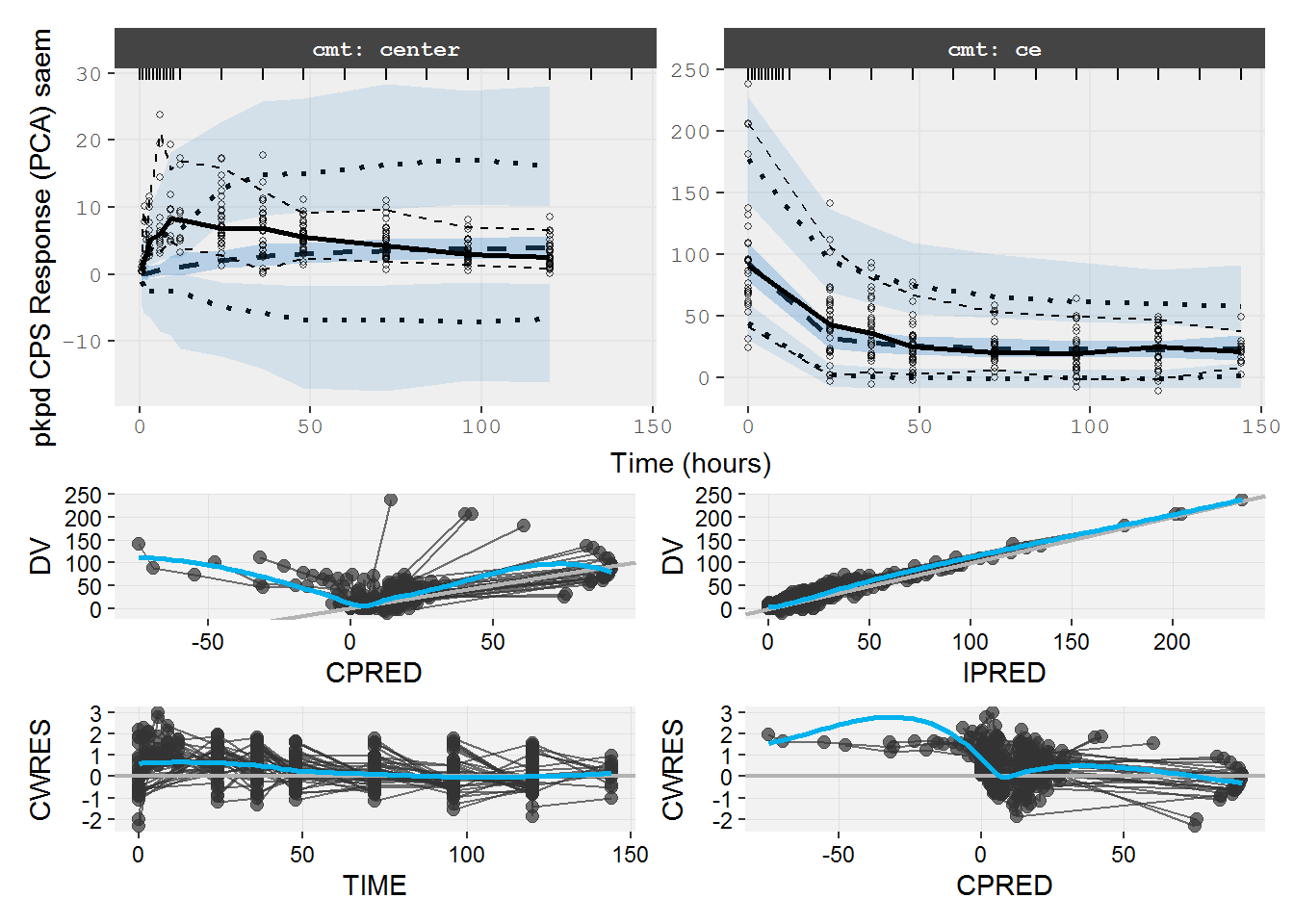
8.2 pkpd.ce.logit Effect CMT PKPD logit
Joint effect CMT logit
pkpd.ce.logit <- function() {
  ini({
    tktr <- log(1)
    tka <- log(1)
    tcl <- log(0.1)
    tv <- log(10)

    eta.ktr ~ 1
    eta.ka ~ 1
    eta.cl ~ 2
    eta.v ~ 1
    eps.pkprop <- 0.1
    eps.pkadd <- 0.1

    poplogit <- 7.5
    tc50 <- log(0.5)
    tkout <- log(0.05)
    te0 <- log(100)

    eta.emax ~ .5
    eta.c50  ~ .5
    eta.kout ~ .5
    eta.e0 ~ .5

    eps.pdadd <- 100
  })
  model({
    ktr <- exp(tktr + eta.ktr)
    ka <- exp(tka + eta.ka)
    cl <- exp(tcl + eta.cl)
    v <- exp(tv + eta.v)

    logit=poplogit+eta.emax
    emax = 1/(1+exp(-logit))
    c50 =  exp(tc50 + eta.c50)
    kout = exp(tkout + eta.kout)
    e0 = exp(te0 + eta.e0)

    cp = center / v
    d/dt(depot) = -ktr * depot
    d/dt(gut) =  ktr * depot -ka * gut
    d/dt(center) =  ka * gut - cl * cp

    d/dt(ce) = kout*(cp - ce)

    effect=e0*(1-emax*ce/(c50+ce))

    cp ~ prop(eps.pkprop) + add(eps.pkadd) | center
    effect ~ add(eps.pdadd) | ce
  })
}
8.2.1 pkpd.fit.CES SAEM
Effect compartment model using the combined PKPD data.
#> __ RxODE-based ODE model _______________________________________________________________________________________________
#> -- Initialization: -----------------------------------------------------------------------------------------------------
#> Fixed Effects ($theta):
#>       tktr        tka        tcl         tv   poplogit       tc50      tkout
#>  0.0000000  0.0000000 -2.3025851  2.3025851  7.5000000 -0.6931472 -2.9957323
#>        te0
#>  4.6051702
#>
#> Omega ($omega):
#>          eta.ktr eta.ka eta.cl eta.v eta.emax eta.c50 eta.kout eta.e0
#> eta.ktr        1      0      0     0      0.0     0.0      0.0    0.0
#> eta.ka         0      1      0     0      0.0     0.0      0.0    0.0
#> eta.cl         0      0      2     0      0.0     0.0      0.0    0.0
#> eta.v          0      0      0     1      0.0     0.0      0.0    0.0
#> eta.emax       0      0      0     0      0.5     0.0      0.0    0.0
#> eta.c50        0      0      0     0      0.0     0.5      0.0    0.0
#> eta.kout       0      0      0     0      0.0     0.0      0.5    0.0
#> eta.e0         0      0      0     0      0.0     0.0      0.0    0.5
#> -- Multiple Endpoint Model ($multipleEndpoint): ------------------------------------------------------------------------
#>       variable                   cmt                   dvid*
#> 1     cp ~ ... cmt='center' or cmt=3 dvid='center' or dvid=1
#> 2 effect ~ ...     cmt='ce' or cmt=4     dvid='ce' or dvid=2
#>
#> -- mu-referencing ($muRefTable): ---------------------------------------------------------------------------------------
#>      theta      eta
#> 1     tktr  eta.ktr
#> 2      tka   eta.ka
#> 3      tcl   eta.cl
#> 4       tv    eta.v
#> 5 poplogit eta.emax
#> 6     tc50  eta.c50
#> 7    tkout eta.kout
#> 8      te0   eta.e0
#>
#> -- Model: --------------------------------------------------------------------------------------------------------------
#>     ktr <- exp(tktr + eta.ktr)
#>     ka <- exp(tka + eta.ka)
#>     cl <- exp(tcl + eta.cl)
#>     v <- exp(tv + eta.v)
#>
#>     logit=poplogit+eta.emax
#>     emax = 1/(1+exp(-logit))
#>     c50 =  exp(tc50 + eta.c50)
#>     kout = exp(tkout + eta.kout)
#>     e0 = exp(te0 + eta.e0)
#>
#>     cp = center / v
#>     d/dt(depot) = -ktr * depot
#>     d/dt(gut) =  ktr * depot -ka * gut
#>     d/dt(center) =  ka * gut - cl * cp
#>
#>     d/dt(ce) = kout*(cp - ce)
#>
#>     effect=e0*(1-emax*ce/(c50+ce))
#>
#>     cp ~ prop(eps.pkprop) + add(eps.pkadd) | center
#>     effect ~ add(eps.pdadd) | ce
#> ________________________________________________________________________________________________________________________
#> [====|====|====|====|====|====|====|====|====|====] 0:00:00
#>
#> [====|====|====|====|====|====|====|====|====|====] 0:00:00
#>
#> [====|====|====|====|====|====|====|====|====|====] 0:00:00
#>
#> [====|====|====|====|====|====|====|====|====|====] 0:00:01
#>
#> [====|====|====|====|====|====|====|====|====|====] 0:00:01
#>
#> [1] "CMT"
#> -- nlmixr SAEM(ODE); OBJF by FOCEi approximation fit -------------------------------------------------------------------
#>
#>          OBJF      AIC      BIC Log-likelihood Condition Number
#> FOCEi 2204.67 3130.364 3209.785      -1546.182         144712.4
#>
#> -- Time (sec pkpd.fit.CES$time): ---------------------------------------------------------------------------------------
#>
#>           saem  setup table cwres covariance other
#> elapsed 143.11 52.095  0.36  52.8       0.08 2.475
#>
#> -- Population Parameters (pkpd.fit.CES$parFixed or pkpd.fit.CES$parFixedDf): -------------------------------------------
#>
#>              Est.     SE %RSE   Back-transformed(95%CI) BSV(CV% or SD)
#> tktr        0.675  0.594 88.1        1.96 (0.613, 6.29)           133.
#> tka        -0.735  0.254 34.5      0.479 (0.291, 0.788)           28.4
#> tcl          -2.2  0.109 4.96     0.111 (0.0892, 0.137)           48.2
#> tv           2.49 0.0838 3.36         12.1 (10.2, 14.2)           32.9
#> eps.pkprop  0.538                                 0.538
#> eps.pkadd  0.0149                                0.0149
#> poplogit     5.92   25.8  435        5.92 (-44.6, 56.5)          0.810
#> tc50       -0.617  0.864  140       0.54 (0.0992, 2.93)           22.9
#> tkout       -5.32  0.772 14.5 0.00488 (0.00107, 0.0222)           40.3
#> te0          4.52 0.0824 1.82            91.7 (78, 108)           45.7
#> eps.pdadd    12.4                                  12.4
#>            Shrink(SD)%
#> tktr            75.5%
#> tka             79.7%
#> tcl             16.7%
#> tv              22.9%
#> eps.pkprop
#> eps.pkadd
#> poplogit        89.3%
#> tc50            59.1%
#> tkout           43.0%
#> te0             3.20%
#> eps.pdadd
#>
#>   Covariance Type (pkpd.fit.CES$covMethod): linFim
#>   Some strong fixed parameter correlations exist (pkpd.fit.CES$cor) :
#>           cor:tka,tktr       cor:tcl,tktr        cor:tv,tktr  cor:poplogit,tktr
#>            -0.638            -0.0355             0.0155            -0.0476
#>      cor:tc50,tktr     cor:tkout,tktr       cor:te0,tktr        cor:tcl,tka
#>           -0.0385            -0.0288            0.00243            -0.0526
#>         cor:tv,tka   cor:poplogit,tka       cor:tc50,tka      cor:tkout,tka
#>             0.118             0.0575             0.0481             0.0375
#>        cor:te0,tka         cor:tv,tcl   cor:poplogit,tcl       cor:tc50,tcl
#>          -0.00459             -0.153             0.0206            -0.0631
#>      cor:tkout,tcl        cor:te0,tcl    cor:poplogit,tv        cor:tc50,tv
#>           -0.0887           -0.00132            0.00557             0.0463
#>       cor:tkout,tv         cor:te0,tv  cor:tc50,poplogit cor:tkout,poplogit
#>             0.103            0.00255              0.892              0.795
#>   cor:te0,poplogit     cor:tkout,tc50       cor:te0,tc50      cor:te0,tkout
#>           -0.0214              0.973            -0.0198            0.00459
#>
#>
#>   No correlations in between subject variability (BSV) matrix
#>   Full BSV covariance (pkpd.fit.CES$omega)
#>     or correlation ( pkpd.fit.CES $omegaR ; diagonals=SDs)
#>   Distribution stats (mean/skewness/kurtosis/p-value) available in $shrink
#>
#> -- Fit Data (object pkpd.fit.CES is a modified tibble): ----------------------------------------------------------------
#> # A tibble: 483 x 38
#>   ID     TIME CMT       DV  PRED    RES   WRES IPRED   IRES  IWRES CPRED   CRES
#>   <fct> <dbl> <fct>  <dbl> <dbl>  <dbl>  <dbl> <dbl>  <dbl>  <dbl> <dbl>  <dbl>
#> 1 1       0.5 center 0.338 0.661 -0.323 -0.493 0.479 -0.140 -0.544 0.639 -0.301
#> 2 1       1   center 0.784 1.87  -1.08  -0.688 1.44  -0.656 -0.847 1.84  -1.06
#> 3 1       2   center 5.09  4.10   0.990  0.344 3.45   1.64   0.887 4.12   0.975
#> # ... with 480 more rows, and 26 more variables: CWRES <dbl>, eta.ktr <dbl>,
#> #   eta.ka <dbl>, eta.cl <dbl>, eta.v <dbl>, eta.emax <dbl>, eta.c50 <dbl>,
#> #   eta.kout <dbl>, eta.e0 <dbl>, depot <dbl>, gut <dbl>, center <dbl>,
#> #   ce <dbl>, ktr <dbl>, ka <dbl>, cl <dbl>, v <dbl>, logit <dbl>, emax <dbl>,
#> #   c50 <dbl>, kout <dbl>, e0 <dbl>, cp <dbl>, effect <dbl>, tad <dbl>,
#> #   dosenum <dbl>
8.2.2 pkpd.fit.CES VPC & GOF
VPC medians do not agree. Note the time trends in the GOF plots (e.g. CPRED vs CWRES).
vpc=myvpc(pkpd.fit.CES,ylab="pkpd CES Response (PCA) saem")
#> [====|====|====|====|====|====|====|====|====|====] 0:00:08

gof=mygof(pkpd.fit.CES)

vpc/gof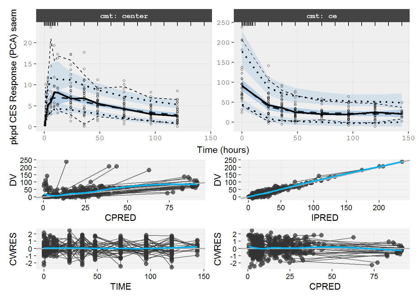
8.3 pkpd.turnover.logit TO PKPD logit
Joint turnover model logit
pkpd.turnover.logit <- function() {
  ini({
    tktr <- log(1)
    tka <- log(1)
    tcl <- log(0.1)
    tv <- log(10)

    eta.ktr ~ 1
    eta.ka ~ 1
    eta.cl ~ 2
    eta.v ~ 1
    eps.pkprop <- 0.1
    eps.pkadd <- 0.1

    poplogit <- 7.5
    tc50 <- log(0.5)
    tkout <- log(0.05)
    te0 <- log(100)

    eta.emax ~ .5
    eta.c50  ~ .5
    eta.kout ~ .5
    eta.e0 ~ .5

    eps.pdadd <- 100
  })
  model({
    ktr <- exp(tktr + eta.ktr)
    ka <- exp(tka + eta.ka)
    cl <- exp(tcl + eta.cl)
    v <- exp(tv + eta.v)

    logit=poplogit+eta.emax
    emax = 1/(1+exp(-logit))
    c50 =  exp(tc50 + eta.c50)
    kout = exp(tkout + eta.kout)
    e0 = exp(te0 + eta.e0)

    cp = center / v
    d/dt(depot) = -ktr * depot
    d/dt(gut) =  ktr * depot -ka * gut
    d/dt(center) =  ka * gut - cl * cp

    effect(0) = e0
    kin = e0*kout
    PD=1-emax*cp/(c50+cp)
    d/dt(effect) = kin*PD -kout*effect

    cp ~ prop(eps.pkprop) + add(eps.pkadd) | center
    effect ~ add(eps.pdadd) | effect
  })
}
8.3.1 pkpd.fit.TOS SAEM
################ Turnover (true) PKPD logit model SAEM ###########
nlmixr(pkpd.turnover.logit) # Show initial estimates and model
#> __ RxODE-based ODE model _______________________________________________________________________________________________
#> -- Initialization: -----------------------------------------------------------------------------------------------------
#> Fixed Effects ($theta):
#>       tktr        tka        tcl         tv   poplogit       tc50      tkout
#>  0.0000000  0.0000000 -2.3025851  2.3025851  7.5000000 -0.6931472 -2.9957323
#>        te0
#>  4.6051702
#>
#> Omega ($omega):
#>          eta.ktr eta.ka eta.cl eta.v eta.emax eta.c50 eta.kout eta.e0
#> eta.ktr        1      0      0     0      0.0     0.0      0.0    0.0
#> eta.ka         0      1      0     0      0.0     0.0      0.0    0.0
#> eta.cl         0      0      2     0      0.0     0.0      0.0    0.0
#> eta.v          0      0      0     1      0.0     0.0      0.0    0.0
#> eta.emax       0      0      0     0      0.5     0.0      0.0    0.0
#> eta.c50        0      0      0     0      0.0     0.5      0.0    0.0
#> eta.kout       0      0      0     0      0.0     0.0      0.5    0.0
#> eta.e0         0      0      0     0      0.0     0.0      0.0    0.5
#> -- Multiple Endpoint Model ($multipleEndpoint): ------------------------------------------------------------------------
#>       variable                   cmt                   dvid*
#> 1     cp ~ ... cmt='center' or cmt=3 dvid='center' or dvid=1
#> 2 effect ~ ... cmt='effect' or cmt=4 dvid='effect' or dvid=2
#>
#> -- mu-referencing ($muRefTable): ---------------------------------------------------------------------------------------
#>      theta      eta
#> 1     tktr  eta.ktr
#> 2      tka   eta.ka
#> 3      tcl   eta.cl
#> 4       tv    eta.v
#> 5 poplogit eta.emax
#> 6     tc50  eta.c50
#> 7    tkout eta.kout
#> 8      te0   eta.e0
#>
#> -- Model: --------------------------------------------------------------------------------------------------------------
#>     ktr <- exp(tktr + eta.ktr)
#>     ka <- exp(tka + eta.ka)
#>     cl <- exp(tcl + eta.cl)
#>     v <- exp(tv + eta.v)
#>
#>     logit=poplogit+eta.emax
#>     emax = 1/(1+exp(-logit))
#>     c50 =  exp(tc50 + eta.c50)
#>     kout = exp(tkout + eta.kout)
#>     e0 = exp(te0 + eta.e0)
#>
#>     cp = center / v
#>     d/dt(depot) = -ktr * depot
#>     d/dt(gut) =  ktr * depot -ka * gut
#>     d/dt(center) =  ka * gut - cl * cp
#>
#>     effect(0) = e0
#>     kin = e0*kout
#>     PD=1-emax*cp/(c50+cp)
#>     d/dt(effect) = kin*PD -kout*effect
#>
#>     cp ~ prop(eps.pkprop) + add(eps.pkadd) | center
#>     effect ~ add(eps.pdadd) | effect
#> ________________________________________________________________________________________________________________________
pkpd.fit.TOS <- nlmixr(pkpd.turnover.logit, data.pkpd, est="saem", control=list(print=0),table=list(cwres=T))
#> [====|====|====|====|====|====|====|====|====|====] 0:00:00
#>
#> [====|====|====|====|====|====|====|====|====|====] 0:00:01
#>
#> [====|====|====|====|====|====|====|====|====|====] 0:00:02
#>
#> [====|====|====|====|====|====|====|====|====|====] 0:00:00
#>
#> [====|====|====|====|====|====|====|====|====|====] 0:00:01
#>
#> [1] "CMT"
if (isplot) plot(pkpd.fit.TOS)
pkpd.fit.TOS
#> -- nlmixr SAEM(ODE); OBJF by FOCEi approximation fit -------------------------------------------------------------------
#>
#>           OBJF     AIC      BIC Log-likelihood Condition Number
#> FOCEi 2327.036 3252.73 3332.151      -1607.365         404302.4
#>
#> -- Time (sec pkpd.fit.TOS$time): ---------------------------------------------------------------------------------------
#>
#>           saem  setup table cwres covariance other
#> elapsed 151.49 65.466  0.36 66.22       0.22 2.464
#>
#> -- Population Parameters (pkpd.fit.TOS$parFixed or pkpd.fit.TOS$parFixedDf): -------------------------------------------
#>
#>              Est.     SE %RSE Back-transformed(95%CI) BSV(CV% or SD)
#> tktr       -0.381  0.166 43.5    0.683 (0.493, 0.945)           33.7
#> tka         -0.01 0.0994  990       0.99 (0.815, 1.2)           20.5
#> tcl         -1.84  0.137 7.44    0.158 (0.121, 0.207)           19.5
#> tv           2.64  0.123 4.67         14.1 (11, 17.9)           29.1
#> eps.pkprop  0.482                               0.482
#> eps.pkadd    2.93                                2.93
#> poplogit     7.06   52.6  746       7.06 (-96.1, 110)          0.862
#> tc50       -0.572  0.338 59.1     0.564 (0.291, 1.09)           65.9
#> tkout       -3.29  0.118 3.59  0.0373 (0.0296, 0.047)           49.7
#> te0          4.51  0.084 1.86        90.9 (77.1, 107)           47.6
#> eps.pdadd    10.7                                10.7
#>            Shrink(SD)%
#> tktr            87.5%
#> tka             89.1%
#> tcl             60.3%
#> tv              48.0%
#> eps.pkprop
#> eps.pkadd
#> poplogit        90.6%
#> tc50            29.0%
#> tkout           19.2%
#> te0             2.40%
#> eps.pdadd
#>
#>   Covariance Type (pkpd.fit.TOS$covMethod): linFim
#>   Some strong fixed parameter correlations exist (pkpd.fit.TOS$cor) :
#>           cor:tka,tktr       cor:tcl,tktr        cor:tv,tktr  cor:poplogit,tktr
#>           -0.0440            -0.0108             0.0605             -0.118
#>      cor:tc50,tktr     cor:tkout,tktr       cor:te0,tktr        cor:tcl,tka
#>           -0.0865             0.0459            0.00561          -0.000269
#>         cor:tv,tka   cor:poplogit,tka       cor:tc50,tka      cor:tkout,tka
#>            0.0283            0.00227            -0.0133            -0.0142
#>        cor:te0,tka         cor:tv,tcl   cor:poplogit,tcl       cor:tc50,tcl
#>         -0.000736             -0.168            -0.0612             -0.439
#>      cor:tkout,tcl        cor:te0,tcl    cor:poplogit,tv        cor:tc50,tv
#>            -0.218            -0.0108             0.0909              0.147
#>       cor:tkout,tv         cor:te0,tv  cor:tc50,poplogit cor:tkout,poplogit
#>             0.165            0.00733              0.792             -0.402
#>   cor:te0,poplogit     cor:tkout,tc50       cor:te0,tc50      cor:te0,tkout
#>           -0.0299             -0.156            -0.0379             0.0804
#>
#>
#>   No correlations in between subject variability (BSV) matrix
#>   Full BSV covariance (pkpd.fit.TOS$omega)
#>     or correlation ( pkpd.fit.TOS $omegaR ; diagonals=SDs)
#>   Distribution stats (mean/skewness/kurtosis/p-value) available in $shrink
#>
#> -- Fit Data (object pkpd.fit.TOS is a modified tibble): ----------------------------------------------------------------
#> # A tibble: 483 x 39
#>   ID     TIME CMT       DV  PRED    RES    WRES IPRED    IRES   IWRES CPRED
#>   <fct> <dbl> <fct>  <dbl> <dbl>  <dbl>   <dbl> <dbl>   <dbl>   <dbl> <dbl>
#> 1 1       0.5 center 0.338 0.456 -0.118 -0.0401 0.405 -0.0664 -0.0226 0.453
#> 2 1       1   center 0.784 1.40  -0.616 -0.202  1.25  -0.465  -0.155  1.39
#> 3 1       2   center 5.09  3.41   1.68   0.470  3.07   2.02    0.614  3.40
#> # ... with 480 more rows, and 28 more variables: CRES <dbl>, CWRES <dbl>,
#> #   eta.ktr <dbl>, eta.ka <dbl>, eta.cl <dbl>, eta.v <dbl>, eta.emax <dbl>,
#> #   eta.c50 <dbl>, eta.kout <dbl>, eta.e0 <dbl>, depot <dbl>, gut <dbl>,
#> #   center <dbl>, effect <dbl>, ktr <dbl>, ka <dbl>, cl <dbl>, v <dbl>,
#> #   logit <dbl>, emax <dbl>, c50 <dbl>, kout <dbl>, e0 <dbl>, cp <dbl>,
#> #   kin <dbl>, PD <dbl>, tad <dbl>, dosenum <dbl>
8.3.2 pkpd.fit.TOS VPC
VPCs look acceptable and no problem visible in the standard GOF plots.
vpc=myvpc(pkpd.fit.TOS,ylab="pkpd TOS Response (PCA) saem")
#> [====|====|====|====|====|====|====|====|====|====] 0:00:03

gof=mygof(pkpd.fit.TOS)

vpc/gof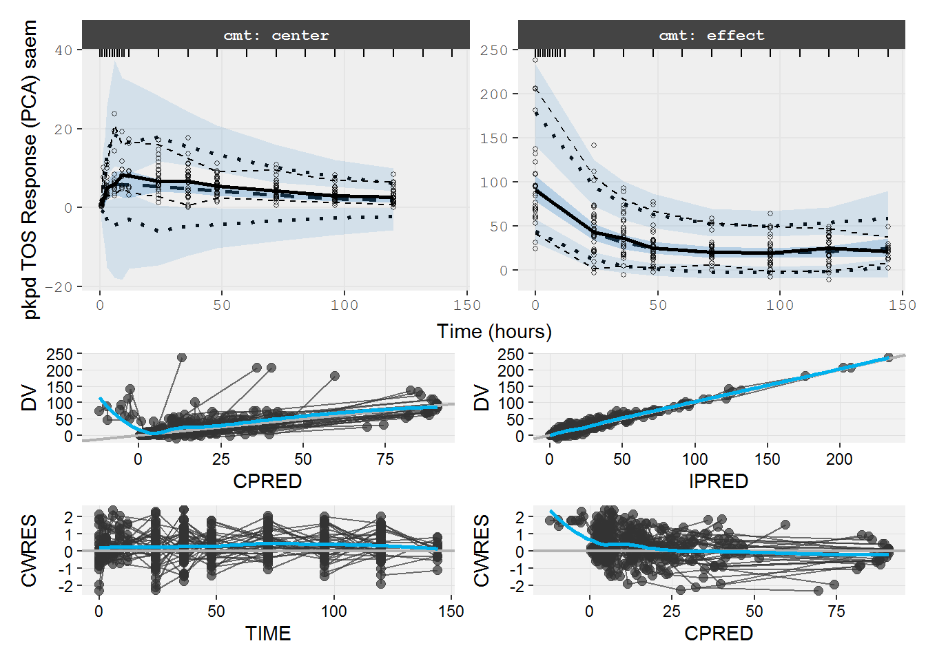
8.4 pkpd.cp.emax Imm Effect PKPD Emax
Joint immediate effect model Emax<1
pkpd.cp.emax <- function() {
  ini({
    tktr <- log(1)
    tka <- log(1)
    tcl <- log(0.1)
    tv <- log(10)

    eta.ktr ~ 1
    eta.ka ~ 1
    eta.cl ~ 2
    eta.v ~ 1
    eps.pkprop <- 0.1
    eps.pkadd <- 0.1

    popemax <- c(0,0.9,0.999)
    tc50 <- log(0.5)
    te0 <- log(100)

    eta.emax ~ .5
    eta.c50  ~ .5
    eta.e0 ~ .5

    eps.pdadd <- 100
  })
  model({
    ktr <- exp(tktr + eta.ktr)
    ka <- exp(tka + eta.ka)
    cl <- exp(tcl + eta.cl)
    v <- exp(tv + eta.v)

    poplogit = log(popemax/(1-popemax))
    logit=poplogit + eta.emax
    emax = 1/(1+exp(-logit))
    c50 =  exp(tc50 + eta.c50)
    e0 = exp(te0 + eta.e0)

    cp = center / v
    d/dt(depot) = -ktr * depot
    d/dt(gut) =  ktr * depot -ka * gut
    d/dt(center) =  ka * gut - cl * cp

    effect=e0*(1-emax*cp/(c50+cp))

    cp ~ prop(eps.pkprop) + add(eps.pkadd) | center
    effect ~ add(eps.pdadd) | effect
  })
}
8.4.1 pkpd.fit.CPF FOCEI
################ Immediate PKPD emax model FOCEI ###########
pkpd.fit.CPF <- nlmixr(pkpd.cp.emax, data.pkpd, est="focei", control=list(print=0,outerOpt="bobyqa",table=list(cwres=T)))
#> [====|====|====|====|====|====|====|====|====|====] 0:00:00
#>
#> [====|====|====|====|====|====|====|====|====|====] 0:00:00
#>
#> [====|====|====|====|====|====|====|====|====|====] 0:00:03
#>
#> [====|====|====|====|====|====|====|====|====|====] 0:00:02
#>
#> [====|====|====|====|====|====|====|====|====|====] 0:00:02
#>
#> [====|====|====|====|====|====|====|====|====|====] 0:00:02
#>
#> [====|====|====|====|====|====|====|====|====|====] 0:00:00
#>
#> [====|====|====|====|====|====|====|====|====|====] 0:00:00
#>
#> [1] "CMT"
#> unhandled error message: EE:lsoda -- at t = 0.00198818 and step size _C(h) = 7.58429e-009, the
#>  corrector convergence failed repeatedly or
#>  with fabs(_C(h)) = hmin
#>  @(lsoda.c:887)
#> unhandled error message: EE:lsoda -- at start of problem, too much accuracy
#>  requested for precision of machine,
#>  suggested scaling factor = 431.47
#>  @(lsoda.c:761)
#> unhandled error message: EE:lsoda -- at start of problem, too much accuracy
#>  requested for precision of machine,
#>  suggested scaling factor = 430.365
#>  @(lsoda.c:761)
#> unhandled error message: EE:lsoda -- at start of problem, too much accuracy
#>  requested for precision of machine,
#>  suggested scaling factor = 64.5623
#>  @(lsoda.c:761)
#> unhandled error message: EE:lsoda -- at start of problem, too much accuracy
#>  requested for precision of machine,
#>  suggested scaling factor = 426.656
#>  @(lsoda.c:761)
#> unhandled error message: EE:lsoda -- at start of problem, too much accuracy
#>  requested for precision of machine,
#>  suggested scaling factor = 368.143
#>  @(lsoda.c:761)
#> unhandled error message: EE:lsoda -- at start of problem, too much accuracy
#>  requested for precision of machine,
#>  suggested scaling factor = 162.742
#>  @(lsoda.c:761)
#> unhandled error message: EE:lsoda -- at start of problem, too much accuracy
#>  requested for precision of machine,
#>  suggested scaling factor = 402.316
#>  @(lsoda.c:761)ll
#> unhandled error message: EE:lsoda -- at start of problem, too much accuracy
#>  requested for precision of machine,
#>  suggested scaling factor = 415.77
#>  @(lsoda.c:761)
#> unhandled error message: EE:lsoda -- at t = 0 and step size _C(h) = 6.97483e-009, the
#>  corrector convergence failed repeatedly or
#>  with fabs(_C(h)) = hmin
#>  @(lsoda.c:887)
#> unhandled error message: EE:lsoda -- at t = 0 and step size _C(h) = 7.58425e-009, the
#>  corrector convergence failed repeatedly or
#>  with fabs(_C(h)) = hmin
#>  @(lsoda.c:887)
#> Error in .fitFun(.ret) :
#>   Evaluation error: Starting values violate bounds.
#> calculating covariance matrix
#> [====|====|====|====|====|====|====|====|====|====] 0:01:56
#> done
if (isplot) plot(pkpd.fit.CPF)
pkpd.fit.CPF
#> -- nlmixr FOCEi (outer: bobyqa) fit ------------------------------------------------------------------------------------
#>
#>           OBJF      AIC      BIC Log-likelihood Condition Number
#> FOCEi 2269.373 3191.068 3262.128      -1578.534         16115.44
#>
#> -- Time (sec pkpd.fit.CPF$time): ---------------------------------------------------------------------------------------
#>
#>          setup optimize covariance table   other
#> elapsed 82.679  116.414    116.414  0.17 524.283
#>
#> -- Population Parameters (pkpd.fit.CPF$parFixed or pkpd.fit.CPF$parFixedDf): -------------------------------------------
#>
#>                Est.     SE %RSE     Back-transformed(95%CI) BSV(CV%)
#> tktr          -1.26  0.327 25.9        0.283 (0.149, 0.538)     11.9
#> tka            2.28   1.76   77           9.83 (0.312, 309)     39.3
#> tcl           -2.17  0.184  8.5       0.114 (0.0795, 0.164)     43.5
#> tv             2.34  0.185 7.89           10.4 (7.24, 14.9)     45.4
#> eps.pkprop    0.317                                   0.317
#> eps.pkadd  0.000289                                0.000289
#> popemax       0.706 0.0537  7.6        0.706 (0.601, 0.812)
#> tc50           -3.5   5.76  164 0.0302 (3.8e-007, 2.4e+003)     323.
#> te0             4.5  0.148 3.29            90.2 (67.5, 121)     41.2
#> eps.pdadd      17.5                                    17.5
#>            Shrink(SD)%
#> tktr            78.5%
#> tka             86.7%
#> tcl             13.1%
#> tv              7.50%
#> eps.pkprop
#> eps.pkadd
#> popemax
#> tc50            90.9%
#> te0             6.30%
#> eps.pdadd
#>
#> -- BSV Covariance (pkpd.fit.CPF$omega): --------------------------------------------------------------------------------
#>             eta.ktr    eta.ka    eta.cl     eta.v eta.emax  eta.c50   eta.e0
#> eta.ktr  0.01414784 0.0000000 0.0000000 0.0000000 0.000000 0.000000 0.000000
#> eta.ka   0.00000000 0.1434983 0.0000000 0.0000000 0.000000 0.000000 0.000000
#> eta.cl   0.00000000 0.0000000 0.1732686 0.0000000 0.000000 0.000000 0.000000
#> eta.v    0.00000000 0.0000000 0.0000000 0.1873769 0.000000 0.000000 0.000000
#> eta.emax 0.00000000 0.0000000 0.0000000 0.0000000 0.179734 0.000000 0.000000
#> eta.c50  0.00000000 0.0000000 0.0000000 0.0000000 0.000000 2.433876 0.000000
#> eta.e0   0.00000000 0.0000000 0.0000000 0.0000000 0.000000 0.000000 0.156704
#>
#>   Not all variables are mu-referenced.
#>   Can also see BSV Correlation (pkpd.fit.CPF$omegaR; diagonals=SDs)
#>   Covariance Type (pkpd.fit.CPF$covMethod): s
#>   Some strong fixed parameter correlations exist (pkpd.fit.CPF$cor) :
#>         cor:tka,tktr     cor:tcl,tktr      cor:tv,tktr cor:popemax,tktr
#>          -0.726            0.262            0.307           -0.250
#>    cor:tc50,tktr     cor:te0,tktr      cor:tcl,tka       cor:tv,tka
#>           0.441           0.0688           -0.191           -0.155
#>  cor:popemax,tka     cor:tc50,tka      cor:te0,tka       cor:tv,tcl
#>          0.0237           -0.516          -0.0349            0.128
#>  cor:popemax,tcl     cor:tc50,tcl      cor:te0,tcl   cor:popemax,tv
#>           0.151            0.439            0.298           -0.116
#>      cor:tc50,tv       cor:te0,tv cor:tc50,popemax  cor:te0,popemax
#>           0.131           -0.144            0.262            0.156
#>     cor:te0,tc50
#>           0.221
#>
#>
#>   Distribution stats (mean/skewness/kurtosis/p-value) available in $shrink
#>   Minimization message (pkpd.fit.CPF$message):
#>     Normal exit from bobyqa
#>
#> -- Fit Data (object pkpd.fit.CPF is a modified tibble): ----------------------------------------------------------------
#> # A tibble: 483 x 36
#>   ID     TIME CMT       DV  PRED    RES   WRES IPRED   IRES  IWRES CPRED   CRES
#>   <fct> <dbl> <fct>  <dbl> <dbl>  <dbl>  <dbl> <dbl>  <dbl>  <dbl> <dbl>  <dbl>
#> 1 1       0.5 center 0.338  1.02 -0.684 -1.21  0.987 -0.649 -2.08   1.02 -0.687
#> 2 1       1   center 0.784  2.15 -1.36  -1.16  2.12  -1.33  -1.99   2.15 -1.37
#> 3 1       2   center 5.09   3.95  1.14   0.532 3.94   1.15   0.921  3.96  1.13
#> # ... with 480 more rows, and 24 more variables: CWRES <dbl>, eta.ktr <dbl>,
#> #   eta.ka <dbl>, eta.cl <dbl>, eta.v <dbl>, eta.emax <dbl>, eta.c50 <dbl>,
#> #   eta.e0 <dbl>, depot <dbl>, gut <dbl>, center <dbl>, ktr <dbl>, ka <dbl>,
#> #   cl <dbl>, v <dbl>, poplogit <dbl>, logit <dbl>, emax <dbl>, c50 <dbl>,
#> #   e0 <dbl>, cp <dbl>, effect <dbl>, tad <dbl>, dosenum <dbl>
8.4.2 pkpd.fit.CPF VPC & GOF
Compiling VPC model…done done (14.89 sec) Quitting from lines 1036-1043 (warf_simtr2_PKPD_vpc_ui_saem_foce_B-18-v3_PDF.Rmd) Error in as.character.factor(df[[col]]) : malformed factor Calls:
#vpc=myvpc(pkpd.fit.CPF,ylab="pkpd CPF Response (PCA) saem")

#gof=mygof(pkpd.fit.CPF)

#vpc/gof
8.5 pkpd.ce.emax Effect CMT PKPD Emax
Joint effect compartment model Emax<1
pkpd.ce.emax <- function() {
  ini({
    tktr <- log(1)
    tka <- log(1)
    tcl <- log(0.1)
    tv <- log(10)

    eta.ktr ~ 1
    eta.ka ~ 1
    eta.cl ~ 2
    eta.v ~ 1
    eps.pkprop <- 0.1
    eps.pkadd <- 0.1

    popemax <- c(0,0.9,0.999)
    tc50 <- log(0.5)
    tkout <- log(0.05)
    te0 <- log(100)

    eta.emax ~ .5
    eta.c50  ~ .5
    eta.kout ~ .5
    eta.e0 ~ .5

    eps.pdadd <- 100
  })
  model({
    ktr <- exp(tktr + eta.ktr)
    ka <- exp(tka + eta.ka)
    cl <- exp(tcl + eta.cl)
    v <- exp(tv + eta.v)

    poplogit = log(popemax/(1-popemax))
    logit=poplogit + eta.emax
    emax = 1/(1+exp(-logit))
    c50 =  exp(tc50 + eta.c50)
    kout = exp(tkout + eta.kout)
    e0 = exp(te0 + eta.e0)

    cp = center / v
    d/dt(depot) = -ktr * depot
    d/dt(gut) =  ktr * depot -ka * gut
    d/dt(center) =  ka * gut - cl * cp

    d/dt(ce) = kout*(cp - ce)

    effect=e0*(1-emax*ce/(c50+ce))

    cp ~ prop(eps.pkprop) + add(eps.pkadd) | center
    effect ~ add(eps.pdadd) | ce
  })
}
8.5.1 pkpd.fit.CEF FOCEI
#> [====|====|====|====|====|====|====|====|====|====] 0:00:00
#>
#> [====|====|====|====|====|====|====|====|====|====] 0:00:00
#>
#> [====|====|====|====|====|====|====|====|====|====] 0:00:01
#>
#> [====|====|====|====|====|====|====|====|====|====] 0:00:02
#>
#> [====|====|====|====|====|====|====|====|====|====] 0:00:01
#>
#> [====|====|====|====|====|====|====|====|====|====] 0:00:02
#>
#> [====|====|====|====|====|====|====|====|====|====] 0:00:00
#>
#> [====|====|====|====|====|====|====|====|====|====] 0:00:00
#>
#> [1] "CMT"
#> intdy -- t = 24 illegal. t not in interval tcur - _C(hu) to tcur
#> intdy -- t = 36 illegal. t not in interval tcur - _C(hu) to tcur
#> intdy -- t = 48 illegal. t not in interval tcur - _C(hu) to tcur
#> intdy -- t = 72 illegal. t not in interval tcur - _C(hu) to tcur
#> intdy -- t = 96 illegal. t not in interval tcur - _C(hu) to tcur
#> intdy -- t = 120 illegal. t not in interval tcur - _C(hu) to tcur
#> unhandled error message: EE:[lsoda] trouble from intdy, itask = 1, tout = 120
#>  @(lsoda.c:689)
#> intdy -- t = 24 illegal. t not in interval tcur - _C(hu) to tcur
#> intdy -- t = 36 illegal. t not in interval tcur - _C(hu) to tcur
#> intdy -- t = 48 illegal. t not in interval tcur - _C(hu) to tcur
#> intdy -- t = 72 illegal. t not in interval tcur - _C(hu) to tcur
#> intdy -- t = 96 illegal. t not in interval tcur - _C(hu) to tcur
#> intdy -- t = 120 illegal. t not in interval tcur - _C(hu) to tcur
#> unhandled error message: EE:[lsoda] trouble from intdy, itask = 1, tout = 120
#>  @(lsoda.c:689)16e
#> intdy -- t = 24 illegal. t not in interval tcur - _C(hu) to tcur
#> intdy -- t = 36 illegal. t not in interval tcur - _C(hu) to tcur
#> intdy -- t = 48 illegal. t not in interval tcur - _C(hu) to tcur
#> intdy -- t = 72 illegal. t not in interval tcur - _C(hu) to tcur
#> intdy -- t = 96 illegal. t not in interval tcur - _C(hu) to tcur
#> intdy -- t = 120 illegal. t not in interval tcur - _C(hu) to tcur
#> unhandled error message: EE:[lsoda] trouble from intdy, itask = 1, tout = 120
#>  @(lsoda.c:689)
#> intdy -- t = 24 illegal. t not in interval tcur - _C(hu) to tcur
#> intdy -- t = 36 illegal. t not in interval tcur - _C(hu) to tcur
#> intdy -- t = 48 illegal. t not in interval tcur - _C(hu) to tcur
#> intdy -- t = 72 illegal. t not in interval tcur - _C(hu) to tcur
#> intdy -- t = 96 illegal. t not in interval tcur - _C(hu) to tcur
#> intdy -- t = 120 illegal. t not in interval tcur - _C(hu) to tcur
#> unhandled error message: EE:[lsoda] trouble from intdy, itask = 1, tout = 120
#>  @(lsoda.c:689)16e
#> intdy -- t = 24 illegal. t not in interval tcur - _C(hu) to tcur
#> intdy -- t = 36 illegal. t not in interval tcur - _C(hu) to tcur
#> intdy -- t = 48 illegal. t not in interval tcur - _C(hu) to tcur
#> intdy -- t = 72 illegal. t not in interval tcur - _C(hu) to tcur
#> intdy -- t = 96 illegal. t not in interval tcur - _C(hu) to tcur
#> intdy -- t = 120 illegal. t not in interval tcur - _C(hu) to tcur
#> unhandled error message: EE:[lsoda] trouble from intdy, itask = 1, tout = 120
#>  @(lsoda.c:689)
#> intdy -- t = 24 illegal. t not in interval tcur - _C(hu) to tcur
#> intdy -- t = 36 illegal. t not in interval tcur - _C(hu) to tcur
#> intdy -- t = 48 illegal. t not in interval tcur - _C(hu) to tcur
#> intdy -- t = 72 illegal. t not in interval tcur - _C(hu) to tcur
#> intdy -- t = 96 illegal. t not in interval tcur - _C(hu) to tcur
#> intdy -- t = 120 illegal. t not in interval tcur - _C(hu) to tcur
#> unhandled error message: EE:[lsoda] trouble from intdy, itask = 1, tout = 120
#>  @(lsoda.c:689)16e
#> intdy -- t = 24 illegal. t not in interval tcur - _C(hu) to tcur
#> intdy -- t = 36 illegal. t not in interval tcur - _C(hu) to tcur
#> intdy -- t = 48 illegal. t not in interval tcur - _C(hu) to tcur
#> intdy -- t = 72 illegal. t not in interval tcur - _C(hu) to tcur
#> intdy -- t = 96 illegal. t not in interval tcur - _C(hu) to tcur
#> intdy -- t = 120 illegal. t not in interval tcur - _C(hu) to tcur
#> unhandled error message: EE:[lsoda] trouble from intdy, itask = 1, tout = 120
#>  @(lsoda.c:689)
#> [====|====|====|====|====|====|====|====|====|====] 0:09:08
#> done
#> -- nlmixr FOCEi (outer: bobyqa) fit ------------------------------------------------------------------------------------
#>
#>           OBJF      AIC      BIC Log-likelihood
#> FOCEi 2136.444 3062.138 3141.559      -1512.069
#>
#> -- Time (sec pkpd.fit.CEF$time): ---------------------------------------------------------------------------------------
#>
#>         setup optimize covariance table  other
#> elapsed 72.23        0          0  0.12 553.66
#>
#> -- Population Parameters (pkpd.fit.CEF$parFixed or pkpd.fit.CEF$parFixedDf): -------------------------------------------
#>
#>              Est. Back-transformed BSV(CV%) Shrink(SD)%
#> tktr        0.496             1.64     25.7      88.2%
#> tka        -0.834            0.434     36.9      67.3%
#> tcl         -2.19            0.111     44.0      10.8%
#> tv           2.41             11.1     41.9      12.1%
#> eps.pkprop  0.344            0.344
#> eps.pkadd   0.135            0.135
#> popemax     0.999            0.999
#> tc50       -0.782            0.457     22.0      59.8%
#> tkout       -5.61          0.00367     38.7      39.9%
#> te0          4.53             93.2     44.7      5.10%
#> eps.pdadd    12.5             12.5
#>
#> -- BSV Covariance (pkpd.fit.CEF$omega): --------------------------------------------------------------------------------
#>             eta.ktr    eta.ka    eta.cl     eta.v eta.emax    eta.c50  eta.kout
#> eta.ktr  0.06388799 0.0000000 0.0000000 0.0000000  0.00000 0.00000000 0.0000000
#> eta.ka   0.00000000 0.1279681 0.0000000 0.0000000  0.00000 0.00000000 0.0000000
#> eta.cl   0.00000000 0.0000000 0.1772143 0.0000000  0.00000 0.00000000 0.0000000
#> eta.v    0.00000000 0.0000000 0.0000000 0.1615624  0.00000 0.00000000 0.0000000
#> eta.emax 0.00000000 0.0000000 0.0000000 0.0000000  2.21256 0.00000000 0.0000000
#> eta.c50  0.00000000 0.0000000 0.0000000 0.0000000  0.00000 0.04745568 0.0000000
#> eta.kout 0.00000000 0.0000000 0.0000000 0.0000000  0.00000 0.00000000 0.1398162
#> eta.e0   0.00000000 0.0000000 0.0000000 0.0000000  0.00000 0.00000000 0.0000000
#>             eta.e0
#> eta.ktr  0.0000000
#> eta.ka   0.0000000
#> eta.cl   0.0000000
#> eta.v    0.0000000
#> eta.emax 0.0000000
#> eta.c50  0.0000000
#> eta.kout 0.0000000
#> eta.e0   0.1824311
#>
#>   Not all variables are mu-referenced.
#>   Can also see BSV Correlation (pkpd.fit.CEF$omegaR; diagonals=SDs)
#>   Covariance Type (pkpd.fit.CEF$covMethod): Boundary issue; Get SEs with getVarCov
#>   Distribution stats (mean/skewness/kurtosis/p-value) available in $shrink
#>   Minimization message (pkpd.fit.CEF$message):
#>     Normal exit from bobyqa
#>
#> -- Fit Data (object pkpd.fit.CEF is a modified tibble): ----------------------------------------------------------------
#> # A tibble: 483 x 39
#>   ID     TIME CMT       DV  PRED    RES   WRES IPRED   IRES  IWRES CPRED   CRES
#>   <fct> <dbl> <fct>  <dbl> <dbl>  <dbl>  <dbl> <dbl>  <dbl>  <dbl> <dbl>  <dbl>
#> 1 1       0.5 center 0.338 0.574 -0.236 -0.592 0.510 -0.172 -0.775 0.571 -0.232
#> 2 1       1   center 0.784 1.69  -0.907 -0.850 1.53  -0.745 -1.37  1.68  -0.900
#> 3 1       2   center 5.09  3.94   1.15   0.494 3.65   1.44   1.14  3.94   1.15
#> # ... with 480 more rows, and 27 more variables: CWRES <dbl>, eta.ktr <dbl>,
#> #   eta.ka <dbl>, eta.cl <dbl>, eta.v <dbl>, eta.emax <dbl>, eta.c50 <dbl>,
#> #   eta.kout <dbl>, eta.e0 <dbl>, depot <dbl>, gut <dbl>, center <dbl>,
#> #   ce <dbl>, ktr <dbl>, ka <dbl>, cl <dbl>, v <dbl>, poplogit <dbl>,
#> #   logit <dbl>, emax <dbl>, c50 <dbl>, kout <dbl>, e0 <dbl>, cp <dbl>,
#> #   effect <dbl>, tad <dbl>, dosenum <dbl>
8.5.2 pkpd.fit.CEF VPC & GOF
vpc=myvpc(pkpd.fit.CEF,ylab="pkpd CEF Response (PCA) saem")
#> [====|====|====|====|====|====|====|====|====|====] 0:00:00
#>
#> [====|====|====|====|====|====|====|====|====|====] 0:00:01
#>
#> [====|====|====|====|====|====|====|====|====|====] 0:00:02
#>
#> [====|====|====|====|====|====|====|====|====|====] 0:00:03
#>
#> [====|====|====|====|====|====|====|====|====|====] 0:00:02
#>
#> [====|====|====|====|====|====|====|====|====|====] 0:00:02
#>
#> [====|====|====|====|====|====|====|====|====|====] 0:00:00
#>
#> [====|====|====|====|====|====|====|====|====|====] 0:00:00
#>
#> [1] "CMT"
#> calculating covariance matrix
#> [====|====|====|====|====|====|====|====|====|====] 0:00:07
#> [====|====|====|====|====|====|====|====|====|====

gof=mygof(pkpd.fit.CEF)

vpc/gof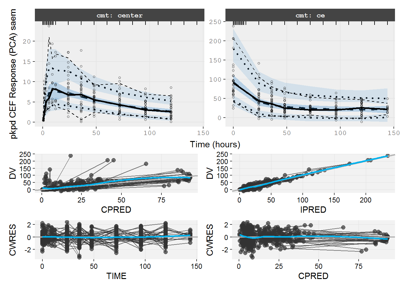
8.6 pkpd.turnover.emax TO PKPD Emax
Joint turnover model Emax<1
pkpd.turnover.emax <- function() {
  ini({
    tktr <- log(1)
    tka <- log(1)
    tcl <- log(0.1)
    tv <- log(10)

    eta.ktr ~ 1
    eta.ka ~ 1
    eta.cl ~ 2
    eta.v ~ 1
    eps.pkprop <- 0.1
    eps.pkadd <- 0.1

    popemax <- c(0,0.9,0.999)
    tc50 <- log(0.5)
    tkout <- log(0.05)
    te0 <- log(100)

    eta.emax ~ .5
    eta.c50  ~ .5
    eta.kout ~ .5
    eta.e0 ~ .5

    eps.pdadd <- 100
  })
  model({
    ktr <- exp(tktr + eta.ktr)
    ka <- exp(tka + eta.ka)
    cl <- exp(tcl + eta.cl)
    v <- exp(tv + eta.v)

    poplogit = log(popemax/(1-popemax))
    logit=poplogit + eta.emax
    emax = 1/(1+exp(-logit))
    c50 =  exp(tc50 + eta.c50)
    kout = exp(tkout + eta.kout)
    e0 = exp(te0 + eta.e0)

    cp = center / v
    d/dt(depot) = -ktr * depot
    d/dt(gut) =  ktr * depot -ka * gut
    d/dt(center) =  ka * gut - cl * cp

    effect(0) = e0
    kin = e0*kout
    PD=1-emax*cp/(c50+cp)
    d/dt(effect) = kin*PD -kout*effect

    cp ~ prop(eps.pkprop) + add(eps.pkadd) | center
    effect ~ add(eps.pdadd) | effect
  })
}
8.6.1 pkpd.fit.TOF FOCEI
################ Turnover (true) PKPD emax model FOCEI ###########
pkpd.fit.TOF <- nlmixr(pkpd.turnover.emax, data.pkpd, est="focei", control=list(print=0,outerOpt="bobyqa",table=list(cwres=T)))
#> [====|====|====|====|====|====|====|====|====|====] 0:00:00
#>
#> [====|====|====|====|====|====|====|====|====|====] 0:00:02
#>
#> [====|====|====|====|====|====|====|====|====|====] 0:00:00
#>
#> [====|====|====|====|====|====|====|====|====|====] 0:00:00
#>
#> [====|====|====|====|====|====|====|====|====|====] 0:00:01
#>
#> [====|====|====|====|====|====|====|====|====|====] 0:00:01
#>
#> [====|====|====|====|====|====|====|====|====|====] 0:00:00
#>
#> [====|====|====|====|====|====|====|====|====|====] 0:00:00
#>
#> [1] "CMT"
#> unhandled error message: EE:lsoda -- at t = 0 and step size _C(h) = 7.58746e-012, the
#>  corrector convergence failed repeatedly or
#>  with fabs(_C(h)) = hmin
#>  @(lsoda.c:887)
#> calculating covariance matrix
#> unhandled error message: EE:lsoda -- at t = 0 and step size _C(h) = 1.13456e-014, the
#>  corrector convergence failed repeatedly or
#>  with fabs(_C(h)) = hmin
#>  @(lsoda.c:887)
#> unhandled error message: EE:lsoda -- at t = 0 and step size _C(h) = 6.47375e-007, the
#>  corrector convergence failed repeatedly or
#>  with fabs(_C(h)) = hmin
#>  @(lsoda.c:887)
#> unhandled error message: EE:lsoda -- at t = 5.52427e-005 and step size _C(h) = 2.10734e-010, the
#>  corrector convergence failed repeatedly or
#>  with fabs(_C(h)) = hmin
#>  @(lsoda.c:887)
#> unhandled error message: EE:lsoda -- at t = 0 and step size _C(h) = 4.70256e-013, the
#>  corrector convergence failed repeatedly or
#>  with fabs(_C(h)) = hmin
#>  @(lsoda.c:887)
#> unhandled error message: EE:lsoda -- at t = 0.579693 and step size _C(h) = 2.04951e-006, the
#>  corrector convergence failed repeatedly or
#>  with fabs(_C(h)) = hmin
#>  @(lsoda.c:887)…Nö=
#> unhandled error message: EE:lsoda -- at t = 0 and step size _C(h) = 2.10734e-010, the
#>  corrector convergence failed repeatedly or
#>  with fabs(_C(h)) = hmin
#>  @(lsoda.c:887)
#> unhandled error message: EE:lsoda -- at t = 60.2022 and step size _C(h) = 3.27922e-005, the
#>  corrector convergence failed repeatedly or
#>  with fabs(_C(h)) = hmin
#>  @(lsoda.c:887)
#> unhandled error message: EE:lsoda -- at t = 6.03157e-008 and step size _C(h) = 4.49387e-016, the
#>  corrector convergence failed repeatedly or
#>  with fabs(_C(h)) = hmin
#>  @(lsoda.c:887)
#> unhandled error message: EE:lsoda -- at t = 0 and step size _C(h) = 6.47376e-007, the
#>  corrector convergence failed repeatedly or
#>  with fabs(_C(h)) = hmin
#>  @(lsoda.c:887)
#> unhandled error message: EE:lsoda -- at t = 8.61749 and step size _C(h) = 3.27922e-005, the
#>  corrector convergence failed repeatedly or
#>  with fabs(_C(h)) = hmin
#>  @(lsoda.c:887)
#> unhandled error message: EE:lsoda -- at t = 0 and step size _C(h) = 1.05367e-010, the
#>  corrector convergence failed repeatedly or
#>  with fabs(_C(h)) = hmin
#>  @(lsoda.c:887)
#> unhandled error message: EE:lsoda -- at t = 60.1951 and step size _C(h) = 3.27922e-005, the
#>  corrector convergence failed repeatedly or
#>  with fabs(_C(h)) = hmin
#>  @(lsoda.c:887)
#> unhandled error message: EE:lsoda -- at t = 0.00707107 and step size _C(h) = 3.27922e-005, the
#>  corrector convergence failed repeatedly or
#>  with fabs(_C(h)) = hmin
#>  @(lsoda.c:887).
#> unhandled error message: EE:lsoda -- at t = 0 and step size _C(h) = 7.46815e-015, the
#>  corrector convergence failed repeatedly or
#>  with fabs(_C(h)) = hmin
#>  @(lsoda.c:887)c:887)
#> unhandled error message: EE:lsoda -- at t = 0 and step size _C(h) = 6.47376e-007, the
#>  corrector convergence failed repeatedly or
#>  with fabs(_C(h)) = hmin
#>  @(lsoda.c:887)
#> unhandled error message: EE:lsoda -- at t = 0 and step size _C(h) = 1.05367e-010, the
#>  corrector convergence failed repeatedly or
#>  with fabs(_C(h)) = hmin
#>  @(lsoda.c:887)
#> unhandled error message: EE:lsoda -- at t = 0 and step size _C(h) = 6.47376e-007, the
#>  corrector convergence failed repeatedly or
#>  with fabs(_C(h)) = hmin
#>  @(lsoda.c:887)
#> unhandled error message: EE:lsoda -- at t = 0 and step size _C(h) = 5.52794e-007, the
#>  corrector convergence failed repeatedly or
#>  with fabs(_C(h)) = hmin
#>  @(lsoda.c:887)
#> unhandled error message: EE:lsoda -- at t = 0 and step size _C(h) = 6.47376e-007, the
#>  corrector convergence failed repeatedly or
#>  with fabs(_C(h)) = hmin
#>  @(lsoda.c:887)c:887)
#> unhandled error message: EE:lsoda -- at t = 0 and step size _C(h) = 1.05367e-010, the
#>  corrector convergence failed repeatedly or
#>  with fabs(_C(h)) = hmin
#>  @(lsoda.c:887)c:887)
#> unhandled error message: EE:lsoda -- at t = 0 and step size _C(h) = 6.47375e-007, the
#>  corrector convergence failed repeatedly or
#>  with fabs(_C(h)) = hmin
#>  @(lsoda.c:887)
#> unhandled error message: EE:lsoda -- at t = 0 and step size _C(h) = 6.47376e-007, the
#>  corrector convergence failed repeatedly or
#>  with fabs(_C(h)) = hmin
#>  @(lsoda.c:887)
#> unhandled error message: EE:lsoda -- at t = 0 and step size _C(h) = 1.05367e-010, the
#>  corrector convergence failed repeatedly or
#>  with fabs(_C(h)) = hmin
#>  @(lsoda.c:887)
#> unhandled error message: EE:lsoda -- at t = 0 and step size _C(h) = 6.47376e-007, the
#>  corrector convergence failed repeatedly or
#>  with fabs(_C(h)) = hmin
#>  @(lsoda.c:887)
#> unhandled error message: EE:lsoda -- at t = 0 and step size _C(h) = 6.47376e-007, the
#>  corrector convergence failed repeatedly or
#>  with fabs(_C(h)) = hmin
#>  @(lsoda.c:887)c:887)
#> unhandled error message: EE:lsoda -- at t = 0 and step size _C(h) = 6.47375e-007, the
#>  corrector convergence failed repeatedly or
#>  with fabs(_C(h)) = hmin
#>  @(lsoda.c:887).c:887)…Nö=
#> unhandled error message: EE:lsoda -- at t = 0 and step size _C(h) = 6.47376e-007, the
#>  corrector convergence failed repeatedly or
#>  with fabs(_C(h)) = hmin
#>  @(lsoda.c:887)c:887)
#> unhandled error message: EE:lsoda -- at t = 0 and step size _C(h) = 6.47375e-007, the
#>  corrector convergence failed repeatedly or
#>  with fabs(_C(h)) = hmin
#>  @(lsoda.c:887)
#> unhandled error message: EE:lsoda -- at t = 0 and step size _C(h) = 6.47376e-007, the
#>  corrector convergence failed repeatedly or
#>  with fabs(_C(h)) = hmin
#>  @(lsoda.c:887)
#> unhandled error message: EE:lsoda -- at t = 0 and step size _C(h) = 6.47376e-007, the
#>  corrector convergence failed repeatedly or
#>  with fabs(_C(h)) = hmin
#>  @(lsoda.c:887)
#> unhandled error message: EE:lsoda -- at t = 0 and step size _C(h) = 1.05367e-010, the
#>  corrector convergence failed repeatedly or
#>  with fabs(_C(h)) = hmin
#>  @(lsoda.c:887)
#> [====|====|====|====|====|====|====|====|====|=
S matrix calculation failed; Switch to R-matrix covariance.
#> ===] 0:08:13
#> done
if (isplot) plot(pkpd.fit.TOF)
pkpd.fit.TOF
#> -- nlmixr FOCEi (outer: bobyqa) fit ------------------------------------------------------------------------------------
#>
#>               OBJF          AIC          BIC Log-likelihood
#> FOCEi 1.811158e+15 1.811158e+15 1.811158e+15  -9.055788e+14
#>
#> -- Time (sec pkpd.fit.TOF$time): ---------------------------------------------------------------------------------------
#>
#>          setup optimize covariance table    other
#> elapsed 67.607   493.37     493.37  0.22 -389.507
#>
#> -- Population Parameters (pkpd.fit.TOF$parFixed or pkpd.fit.TOF$parFixedDf): -------------------------------------------
#>
#>               Est. Back-transformed BSV(CV%) Shrink(SD)%
#> tktr       -0.0187            0.981     113.      74.5%
#> tka         -0.026            0.974     106.      73.8%
#> tcl          -2.33           0.0976     113.      73.3%
#> tv            2.31               10     71.9      4.58%
#> eps.pkprop    0.14             0.14
#> eps.pkadd    0.116            0.116
#> popemax      0.854            0.854
#> tc50        -0.699            0.497     79.2      2.85%
#> tkout        -2.98           0.0506     74.2     -627.%
#> te0           4.54             93.9     59.1      48.0%
#> eps.pdadd       47               47
#>
#> -- BSV Covariance (pkpd.fit.TOF$omega): --------------------------------------------------------------------------------
#>            eta.ktr    eta.ka    eta.cl     eta.v  eta.emax   eta.c50  eta.kout
#> eta.ktr  0.8246359 0.0000000 0.0000000 0.0000000 0.0000000 0.0000000 0.0000000
#> eta.ka   0.0000000 0.7518864 0.0000000 0.0000000 0.0000000 0.0000000 0.0000000
#> eta.cl   0.0000000 0.0000000 0.8201897 0.0000000 0.0000000 0.0000000 0.0000000
#> eta.v    0.0000000 0.0000000 0.0000000 0.4165251 0.0000000 0.0000000 0.0000000
#> eta.emax 0.0000000 0.0000000 0.0000000 0.0000000 0.4649877 0.0000000 0.0000000
#> eta.c50  0.0000000 0.0000000 0.0000000 0.0000000 0.0000000 0.4866589 0.0000000
#> eta.kout 0.0000000 0.0000000 0.0000000 0.0000000 0.0000000 0.0000000 0.4390234
#> eta.e0   0.0000000 0.0000000 0.0000000 0.0000000 0.0000000 0.0000000 0.0000000
#>             eta.e0
#> eta.ktr  0.0000000
#> eta.ka   0.0000000
#> eta.cl   0.0000000
#> eta.v    0.0000000
#> eta.emax 0.0000000
#> eta.c50  0.0000000
#> eta.kout 0.0000000
#> eta.e0   0.2999657
#>
#>   Not all variables are mu-referenced.
#>   Can also see BSV Correlation (pkpd.fit.TOF$omegaR; diagonals=SDs)
#>   Covariance Type (pkpd.fit.TOF$covMethod): failed
#>   Distribution stats (mean/skewness/kurtosis/p-value) available in $shrink
#>   Minimization message (pkpd.fit.TOF$message):
#>     Normal exit from bobyqa
#>
#> -- Fit Data (object pkpd.fit.TOF is a modified tibble): ----------------------------------------------------------------
#> # A tibble: 483 x 40
#>   ID     TIME CMT       DV  PRED    RES   WRES IPRED   IRES  IWRES CPRED   CRES
#>   <fct> <dbl> <fct>  <dbl> <dbl>  <dbl>  <dbl> <dbl>  <dbl>  <dbl> <dbl>  <dbl>
#> 1 1       0.5 center 0.338 0.863 -0.525 -0.485 0.870 -0.531 -3.16  0.863 -0.525
#> 2 1       1   center 0.784 2.54  -1.75  -0.628 2.56  -1.77  -4.71  2.54  -1.75
#> 3 1       2   center 5.09  5.74  -0.649 -0.129 5.77  -0.676 -0.829 5.74  -0.650
#> # ... with 480 more rows, and 28 more variables: CWRES <dbl>, eta.ktr <dbl>,
#> #   eta.ka <dbl>, eta.cl <dbl>, eta.v <dbl>, eta.emax <dbl>, eta.c50 <dbl>,
#> #   eta.kout <dbl>, eta.e0 <dbl>, depot <dbl>, gut <dbl>, center <dbl>,
#> #   effect <dbl>, ktr <dbl>, ka <dbl>, cl <dbl>, v <dbl>, poplogit <dbl>,
#> #   logit <dbl>, emax <dbl>, c50 <dbl>, kout <dbl>, e0 <dbl>, cp <dbl>,
#> #   kin <dbl>, PD <dbl>, tad <dbl>, dosenum <dbl>
8.6.2 pkpd.fit.TOF VPC
vpc=myvpc(pkpd.fit.TOF,ylab="pkpd TOF Response (PCA) saem")
#> [====|====|====|====|====|====|====|====|====|====] 0:00:00
#>
#> [====|====|====|====|====|====|====|====|====|====] 0:00:02
#>
#> [====|====|====|====|====|====|====|====|====|====] 0:00:00
#>
#> [====|====|====|====|====|====|====|====|====|====] 0:00:00
#>
#> [====|====|====|====|====|====|====|====|====|====] 0:00:01
#>
#> [====|====|====|====|====|====|====|====|====|====] 0:00:01
#>
#> [====|====|====|====|====|====|====|====|====|====] 0:00:00
#>
#> [====|====|====|====|====|====|====|====|====|====] 0:00:00
#>
#> [1] "CMT"
#> calculating covariance matrix
#> unhandled error message: EE:lsoda -- at t = 105.035 and step size _C(h) = 1.39265e-008, the
#>  error test failed repeatedly or
#>  with fabs(_C(h)) = hmin
#>  @(lsoda.c:884)
#> [====|====|====|====|====|====|====|====|====|=
S matrix calculation failed; Switch to R-matrix covariance.
#> ===] 0:00:20
#> [====|====|====|====|====|====|====|====|====|====

gof=mygof(pkpd.fit.TOF)

vpc/gof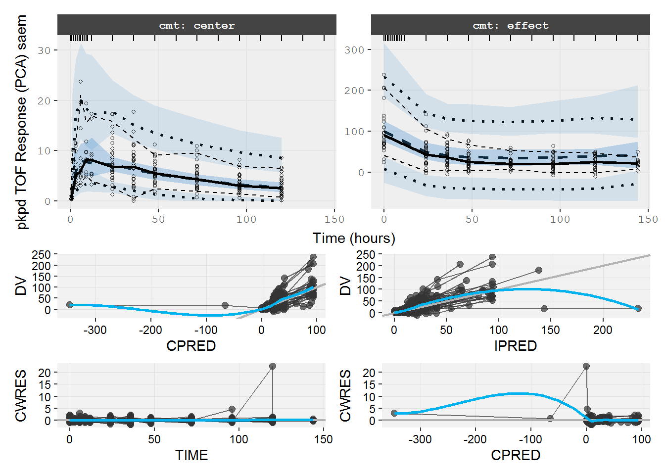
9 Rmarkdown
Output created: warf_simtr_PKPD_vpc_ui_saem_foce_B-18-v3_PDF.html